Aggregation: from surviving trials to parameters

Screening decides which trials survive. Aggregation decides what the survivors are summarised as, and the two fail differently, which is why rtprep keeps them apart. The same trials summarised two ways give two different sets of summary statistics, and the parameters follow from those. This article walks through rt_summary()’s methods and its weights, the accuracy correction that goes with the mixture route, the ez_ddm() inversion and its scaling convention, and then puts five routes side by side on rt_example, whose cells carry the drift they were generated from.

library(rtprep)
library(dplyr)
library(ggplot2)

What `rt_summary()` returns

The EZ-diffusion equations need three things per cell: the mean response time, its variance, and the proportion correct. rt_summary() returns the first two and the counts behind the third, one row per call, so it fits inside reframe() the way rt_screen() fits inside mutate():

p3_hard <- rt_example |>
  filter(id == "p3", condition == "hard")

rt_summary(p3_hard$rt, p3_hard$response)
#>     mean_rt    var_rt n_upper n_trials contaminant_prop
#> 1 0.6412949 0.1046185      84      100               NA

contaminant_prop is NA for every method but "mixture", which is the only one that estimates it. version = "4par" summarises the two response boundaries separately, for the version of the model that lets the starting point sit off centre:

rt_summary(p3_hard$rt, p3_hard$response, version = "4par")
#>   mean_rt_upper mean_rt_lower var_rt_upper var_rt_lower n_upper n_trials
#> 1     0.6292822     0.7043615   0.06340244    0.3346047      84      100
#>   contaminant_prop_upper contaminant_prop_lower
#> 1                     NA                     NA

One caveat carries over from bmm. A trial whose response is missing belongs to neither boundary and is left out of n_upper, but it still counts towards n_trials, so the ratio understates accuracy when responses are missing. Drop those trials before aggregating if that matters.

Robust moments

method = "robust" replaces the mean with the median and the variance with a robust spread: the interquartile range divided by 1.349, squared, or the median absolute deviation. This is robustness at the level of the statistic, after Chávez De la Peña et al. (2026): no trial is removed, and a contaminant in the tail moves the median very little and the interquartile range not at all.

moments <- bind_rows(
  simple = rt_summary(p3_hard$rt, p3_hard$response),
  robust_iqr = rt_summary(p3_hard$rt, p3_hard$response, method = "robust"),
  robust_mad = rt_summary(
    p3_hard$rt, p3_hard$response, method = "robust", robust_scale = "mad"
  ),
  .id = "method"
)
moments |>
  select(method, mean_rt, var_rt)
#>       method   mean_rt     var_rt
#> 1     simple 0.6412949 0.10461851
#> 2 robust_iqr 0.5620000 0.03434441
#> 3 robust_mad 0.5620000 0.03714794

The median sits well below the mean, as it does for any right-skewed distribution, and the IQR-based robust variance is 33% of the sample variance. Those are not corrections for contamination; they are different statistics, and they feed the same equations. The last section puts the four routes side by side.

Trimmed and Winsorized moments

method = "trimmed" takes the mean of the middle 1 - 2 * trim of the trials; method = "winsorized" replaces the extremes with the nearest surviving value instead of dropping them, and takes the mean of that. Both read their variance off the Winsorized sample, so the count stays at n_trials either way and only the pull of the extremes is removed.

bind_rows(
  simple = rt_summary(p3_hard$rt, p3_hard$response),
  trimmed = rt_summary(
    p3_hard$rt, p3_hard$response, method = "trimmed", trim = 0.1
  ),
  winsorized = rt_summary(
    p3_hard$rt, p3_hard$response, method = "winsorized", trim = 0.1
  ),
  .id = "method"
) |>
  select(method, mean_rt, var_rt, n_trials)
#>       method   mean_rt     var_rt n_trials
#> 1     simple 0.6412949 0.10461851      100
#> 2    trimmed 0.5861795 0.05100875      100
#> 3 winsorized 0.6043436 0.05100875      100

This is still statistic-level robustness, not trimming in the screening sense: no trial is excluded from the analysis, n_trials does not move, and nothing is written down about which trials were unusual. A reader cannot tell from the output which trials were trimmed, because the answer is “the extreme 10% of this cell, by construction” rather than “the ones a criterion flagged”.

One thing about the variance is worth stating, because it is easy to get wrong. The Winsorized variance estimates the variance of the Winsorized distribution, which is too small for ez_ddm(): the EZ equations read var_rt as a moment of the response time distribution the decision process produced. rt_summary() therefore rescales it. The familiar (1 - 2 * trim)^2 divisor of Tukey and McLaughlin is not what it uses, because that divisor targets the variance of the trimmed mean and returns a variance that runs roughly 6% high at trim = 0.1 and 14% high at trim = 0.2 when the data are normal; rtprep uses the normal-consistency constant, which lands within half a percent. If you compare var_rt against a hand-computed Winsorized variance and the two differ, this is why.

Mixture moments

method = "mixture" fits the same contaminant mixture rule_mixture() fits, then reads the mean and variance off the fitted core rather than off the data. A trial the uniform component owns contributes nothing to the moments, and the estimated contaminant proportion comes back alongside them. This is the summary-level version of modelling the contaminant instead of deleting it:

bind_rows(lapply(c("exgaussian", "lognormal", "invgaussian"), function(core) {
  rt_summary(
    p3_hard$rt, p3_hard$response, method = "mixture", distribution = core
  ) |>
    mutate(distribution = core, .before = 1)
})) |>
  select(distribution, mean_rt, var_rt, contaminant_prop)
#>   distribution   mean_rt     var_rt contaminant_prop
#> 1   exgaussian 0.6182632 0.06133313       0.01744821
#> 2    lognormal 0.6076591 0.04476575       0.02722565
#> 3  invgaussian 0.6092693 0.04484182       0.02756894

The ... arguments go to the fit as in rule_mixture(), with the same defaults, including maxit = 500 where bmm::ezdm_summary_stats() uses 100. When the fit fails the moments fall back to the robust ones with a warning, as in bmm. That differs from rt_screen(), where the analogous failure keeps every trial, and the difference is deliberate: a screen that cannot be evaluated should remove nothing, but a summary still has to return a number.

rt_summary(p3_hard$rt, p3_hard$response, method = "mixture", maxit = 2)
#> Warning: The mixture fit did not converge; using robust moments instead.
#>   mean_rt     var_rt n_upper n_trials contaminant_prop
#> 1   0.562 0.03434441      84      100               NA

Weights: the other way of not letting contaminants count

The mixture screen’s .prob can go into rt_summary() as a weight vector instead of through a threshold. Weighted moments let a doubtful trial contribute a little, where mixture moments let a trial the uniform component owns contribute nothing at all. The two are different models of the same doubt, and the package refuses to combine them:

screened <- rt_screen(p3_hard$rt, rule_mixture("lognormal"))

rt_summary(p3_hard$rt, p3_hard$response, weights = screened$.prob)
#>     mean_rt     var_rt n_upper n_trials contaminant_prop
#> 1 0.6096456 0.05326504      84      100               NA

try(rt_summary(
  p3_hard$rt, p3_hard$response, weights = screened$.prob, method = "mixture"
))
#> Error : 'weights' is defined for method = "simple" only. Every other method already carries its own answer to contamination, and combining two of them is an error rather than a convenience.

The weighted variance uses the reliability-weight denominator \(\sum w - \sum w^2 / \sum w\), which reduces to \(n - 1\) when the weights are equal. Frequency weights would use \(\sum w - 1\) and are the wrong model, because .prob is a probability, not a count. The same reasoning governs min_trials: with weights, the comparison uses Kish’s effective sample size \((\sum w)^2 / \sum w^2\), so two unit weights among ninety-eight zeros count as two trials, and the moments come back NA rather than as noise:

two_trials <- c(rep(1, 2), rep(0, 98))
rt_summary(p3_hard$rt, p3_hard$response, weights = two_trials)
#>   mean_rt var_rt n_upper n_trials contaminant_prop
#> 1      NA     NA      84      100               NA

Correcting the accuracy counts

Mixture moments take the contaminants out of the response times, but the accuracy counts still include them. adjust_accuracy() removes the estimated contaminants from the counts on the assumption that they respond correctly at guess_rate. It is stochastic by design: how many trials were contaminants, and how many of those happened to be correct, are both binomial draws, and a point estimate would understate that uncertainty. There is no set.seed() inside the package, so the seed is yours:

set.seed(2026094)
adjust_accuracy(n_upper = 84, n_trials = 100, contaminant_prop = 0.10)
#>   n_upper_adj n_trials_adj
#> 1          81           91

# NA or zero leaves the counts alone, so the column of a summary table
# drops in as it is
adjust_accuracy(n_upper = 84, n_trials = 100, contaminant_prop = NA)
#>   n_upper_adj n_trials_adj
#> 1          84          100

The function is vectorised over its rows and draws each row independently, so it takes the columns of a summary table directly. For a single row the two draws are made in the same order as bmm::adjust_ezdm_accuracy(), and the two functions agree draw for draw from the same seed.

`ez_ddm()` and the scaling constant

ez_ddm() is the closed-form inversion of Wagenmakers, van der Maas, and Grasman (2007): mean, variance, and accuracy in; drift, bound, and non-decision time out. It is exported so that the whole chain from screening to parameters runs with rtprep alone. The one argument that needs a sentence is s. Wagenmakers et al. fix the diffusion coefficient at 0.1, rtprep at 1, and the choice is a units convention rather than a modelling one: drift and bound scale linearly with s, non-decision time does not. Their worked example under both conventions:

bind_rows(
  wagenmakers = ez_ddm(
    mean_rt = 0.723, var_rt = 0.112, accuracy = 0.802, n_trials = 100, s = 0.1
  ),
  rtprep = ez_ddm(
    mean_rt = 0.723, var_rt = 0.112, accuracy = 0.802, n_trials = 100
  ),
  .id = "convention"
)
#>    convention      drift     bound     ndt edge_corrected
#> 1 wagenmakers 0.09993853 0.1399702 0.30003          FALSE
#> 2      rtprep 0.99938526 1.3997020 0.30003          FALSE

A drift of 0.1 at s = 0.1 and a drift of 1 at s = 1 describe the same process. Anything compared across packages or papers has to be on one scale first; bmm uses 1 as well.

The equations divide by the logit of accuracy and break down at 0, 0.5, and 1. The published edge correction moves the offending value by \(1 / (2n)\), and ez_ddm() applies it silently, because a warning per cell would bury a simulation run. Which rows it touched comes back as a column, so that it survives subsetting and the dplyr verbs:

edges <- ez_ddm(
  mean_rt = 0.5, var_rt = 0.02, accuracy = c(1, 0.5, 0.9), n_trials = 50
)
edges
#>        drift     bound       ndt edge_corrected
#> 1 3.17897186 1.4454736 0.2771978           TRUE
#> 2 0.04805879 0.8324249 0.3267903           TRUE
#> 3 2.17111652 1.0120252 0.3135475          FALSE

A cell at perfect accuracy gets a drift of 3.2 rather than infinity, and edge_corrected is the flag to count in a results table.

Four routes on `rt_example`

The routes above are alternatives to trimming, not additions to it. Five pipelines on rt_example, each applied per cell: no preprocessing, the ±2.5 SD trim with simple moments, robust moments on all trials, a 10% trimmed mean on all trials, and mixture moments on all trials with the accuracy counts adjusted. Only the second removes a trial; the rest change the statistic. Each ends in ez_ddm(), and the data carry the drift each cell was generated from:

summarise_cells <- function(data, ...) {
  data |>
    reframe(rt_summary(rt, response, ...), .by = c(id, condition))
}

routes <- bind_rows(
  none = summarise_cells(rt_example),
  sd_trim = rt_example |>
    filter(rt_keep(rt, rule_sd(2.5), .by = list(id, condition))) |>
    summarise_cells(),
  robust = summarise_cells(rt_example, method = "robust"),
  trimmed = summarise_cells(rt_example, method = "trimmed", trim = 0.1),
  mixture = summarise_cells(
    rt_example, method = "mixture", distribution = "lognormal"
  ),
  .id = "route"
)
#> sd(2.5, mean, sd): dropped 26 of 800 trials (3.2%)

set.seed(2026094)
estimates <- routes |>
  mutate(adjust_accuracy(n_upper, n_trials, contaminant_prop)) |>
  mutate(ez_ddm(mean_rt, var_rt, n_upper_adj / n_trials_adj, n_trials_adj)) |>
  left_join(
    distinct(rt_example, id, condition, true_drift, contam_rate),
    by = c("id", "condition")
  ) |>
  mutate(
    route = factor(
      route,
      levels = c("none", "sd_trim", "robust", "trimmed", "mixture")
    ),
    error = drift - true_drift
  )

estimates |>
  summarise(
    mean_error = mean(error),
    mean_abs_error = mean(abs(error)),
    .by = route
  )
#>     route  mean_error mean_abs_error
#> 1    none -0.35712935     0.35712935
#> 2 sd_trim -0.05790345     0.13121618
#> 3  robust  0.01250529     0.07332629
#> 4 trimmed -0.13078766     0.17284020
#> 5 mixture  0.35405639     0.37006909

ggplot(estimates, aes(x = condition, y = drift, colour = route)) +
  geom_point(
    aes(y = true_drift), shape = 95, size = 8, colour = "black"
  ) +
  geom_point(position = position_dodge(width = 0.5), size = 2) +
  scale_colour_manual(values = okabe_ito[c(8, 1, 3, 6, 2)]) +
  facet_wrap(~id, nrow = 1) +
  labs(x = NULL, y = "Estimated drift", colour = NULL) +
  theme_minimal() +
  theme(legend.position = "bottom")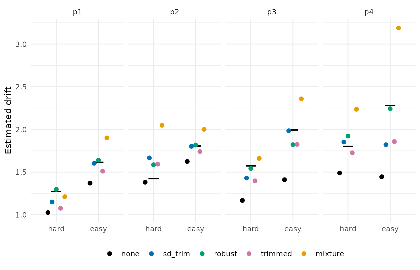

Dot plot of the estimated drift of each participant and condition under five aggregation routes, with the true drift drawn as a black bar in each cell.

The table is each route’s mean signed and mean absolute error against the generating drift over the eight cells; the figure puts the five estimates of every cell next to its true drift. Two mechanical differences separate the mixture route from the other four, and both enter ez_ddm() in the same direction: its variance is read off the fitted core rather than the sample, and adjust_accuracy() raises the proportion correct; a smaller variance and a higher accuracy both raise the drift.

Eight cells of 100 trials cannot rank five pipelines, and this page does not try. What they show is that the same trials summarised five ways give five drift estimates per cell, and the route column is the whole difference between them. The ground-truth article carries the same chain through on data matched to a task of your own, with a perfect-exclusion oracle as the ceiling.

Differences from `bmm`

bmm::ezdm_summary_stats() returns the same columns under the same names, and the two functions are compared over the full grid of methods, versions, and cores in rtprep’s test suite. Three defaults differ. rt_summary() defaults to method = "simple" where bmm defaults to "mixture", because a package about preprocessing choices should not make one of them silently. The mixture route defaults to maxit = 500 where bmm uses 100. And for version = "4par" with mixture moments, the contaminant bounds are resolved once on the pooled response times before the split, so that the two halves are fitted against the same uniform component. The correspondence between the two packages, function by function, is the subject of its own article.

What rt_summary() returns