Comparing rules: what a different choice would have removed

The question rtprep exists to make askable is what a different preprocessing choice would have removed. It is normally unanswerable because every implementation returns a different shape: a trimmed data frame here, a vector of probabilities there, a set of summary statistics somewhere else. With one return shape the comparison is one call, and this article is about that call: what screen_compare() returns, which of its two agreement measures answers which question, how to see what each rule removed and why, and how to tabulate the roster’s settings and realised drop rates from the result object.

library(rtprep)
library(dplyr)
library(ggplot2)

One call, several tables

screen_compare() takes a named list of rules and applies each one with the same grouping, policy, and threshold. The get-started vignette runs a five-rule roster; this one adds the accuracy chart, which needs response, and uses the lognormal mixture:

roster <- list(
  cutoff = rule_cutoff(0.18, 3),
  sd = rule_sd(2.5),
  mad = rule_mad(2.5),
  recursive = rule_recursive("modified"),
  mixture = rule_mixture("lognormal"),
  ewma = rule_ewma()
)

cmp <- screen_compare(
  rt_example$rt, roster,
  response = rt_example$response,
  .by = list(rt_example$id, rt_example$condition)
)
cmp
#> <rtprep comparison> 800 trials, 6 rules
#> 
#>   cutoff                       dropped   0.0%
#>   sd                           dropped   3.2%
#>   mad                          dropped  11.4%
#>   recursive                    dropped   4.1%
#>   mixture                      dropped   4.0%
#>   ewma                         dropped   7.8%
#> 
#>   least agreement: mad vs ewma, 80.9% of decisions (Jaccard 0.00)

The print method gives the overall drop rate per rule and the pair that agrees least. Behind it sit three matrices with one row per trial and one column per rule, and three tables:

names(cmp)
#> [1] "keep"      "prob"      "reason"    "drops"     "agreement" "fits"     
#> [7] "n_trials"  "rules"     "call"
dim(cmp$keep)
#> [1] 800   6

keep, prob, and reason are the per-trial columns of rt_screen() stacked side by side; drops counts what each rule removed per group, with a column per reason; agreement compares every pair; fits stacks each rule’s per-group diagnostics with a .rule column. summary(cmp) prints the drops and the agreement in full.

Agreement and Jaccard answer different questions

cmp$agreement
#>       rule_x    rule_y   agree   jaccard n_only_x n_only_y n_both
#> 1     cutoff        sd 0.96750 0.0000000        0       26      0
#> 2     cutoff       mad 0.88625 0.0000000        0       91      0
#> 3     cutoff recursive 0.95875 0.0000000        0       33      0
#> 4     cutoff   mixture 0.96000 0.0000000        0       32      0
#> 5     cutoff      ewma 0.92250 0.0000000        0       62      0
#> 6         sd       mad 0.91875 0.2857143        0       65     26
#> 7         sd recursive 0.99125 0.7878788        0        7     26
#> 8         sd   mixture 0.99000 0.7575758        1        7     25
#> 9         sd      ewma 0.89000 0.0000000       26       62      0
#> 10       mad recursive 0.92750 0.3626374       58        0     33
#> 11       mad   mixture 0.92625 0.3516484       59        0     32
#> 12       mad      ewma 0.80875 0.0000000       91       62      0
#> 13 recursive   mixture 0.99875 0.9696970        1        0     32
#> 14 recursive      ewma 0.88125 0.0000000       33       62      0
#> 15   mixture      ewma 0.88250 0.0000000       32       62      0

agree is the share of trials on which two rules made the same decision. jaccard is the overlap of the two sets of removed trials: the size of their intersection over the size of their union. The two diverge exactly where it matters, and a constructed pair shows the extreme. On one cell, a cutoff that removes only the fastest 2% and a cutoff that removes only the slowest 2% never remove the same trial:

p3_hard <- rt_example |>
  filter(id == "p3", condition == "hard")

edges <- screen_compare(
  p3_hard$rt,
  list(
    fast_only = rule_cutoff(min = quantile(p3_hard$rt, 0.02)),
    slow_only = rule_cutoff(max = quantile(p3_hard$rt, 0.98))
  )
)
edges$agreement
#>      rule_x    rule_y agree jaccard n_only_x n_only_y n_both
#> 1 fast_only slow_only  0.96       0        2        2      0

They agree on 96% of decisions and overlap not at all. Agreement alone would call them interchangeable, and in the roster above the same thing happens to every pair that includes the chart: it agrees with the other rules on 81% of decisions or more and shares no removed trial with any of them, because it cuts from below and the rest cut from above. The other reading is the recursive criterion against the mixture, which agree on 99.9% of decisions and overlap at 0.97: two rules from different families that removed almost the same trials.

One more case is deliberate. When neither rule removed anything there is no overlap to compute, and jaccard is NA rather than 1, because calling an empty comparison a perfect match would make it look like agreement:

screen_compare(
  p3_hard$rt,
  list(wide = rule_cutoff(0.1, 5), none = rule_none())
)$agreement
#>   rule_x rule_y agree jaccard n_only_x n_only_y n_both
#> 1   wide   none     1      NA        0        0      0

What each rule removed, and why

The drops table has one row per rule and group, and a column for every reason any rule gave. Summing over groups shows the composition of each rule’s removals:

cmp$drops |>
  summarise(
    across(c(n_dropped, too_fast, too_slow, contaminant), sum),
    .by = .rule
  )
#>       .rule n_dropped too_fast too_slow contaminant
#> 1    cutoff         0        0        0           0
#> 2        sd        26        0       26           0
#> 3       mad        91        0       91           0
#> 4 recursive        33        0       33           0
#> 5   mixture        32        0        0          32
#> 6      ewma        62       62        0           0

The SD and MAD criteria and the recursive criterion removed nothing but slow trials, and the cutoff removed nothing at all. The chart removed nothing but fast ones. The mixture’s reason is "contaminant", because a posterior has no side. Those are three different bets about where the contamination sits, and the table shows which one a rule made without the truth being consulted. Per group the drops vary more than the totals suggest; the chart’s rate runs from 2% to 22% across the eight cells, which is its lag showing per participant.

The plot

The plot method draws the drop rates and returns a ggplot when ggplot2 is installed, with a base-graphics fallback when it is not, so the usual additions apply:

plot(cmp) +
  labs(title = "Proportion of trials each rule removed") +
  theme_minimal()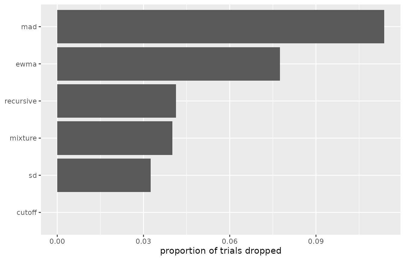

#> NULL

The agreement table draws as a tile plot of the Jaccard overlap, which makes the two clusters visible at once: the rules that cut from above overlap with each other and with nothing else.

cmp$agreement |>
  mutate(
    rule_x = factor(rule_x, levels = names(roster)),
    rule_y = factor(rule_y, levels = rev(names(roster)))
  ) |>
  ggplot(aes(rule_x, rule_y, fill = jaccard)) +
  geom_tile(colour = "white") +
  geom_text(aes(label = round(jaccard, 2)), size = 3.5) +
  scale_fill_gradient(low = "grey92", high = okabe_ito[1], limits = c(0, 1)) +
  labs(x = NULL, y = NULL, fill = "Jaccard") +
  theme_minimal() +
  theme(panel.grid = element_blank())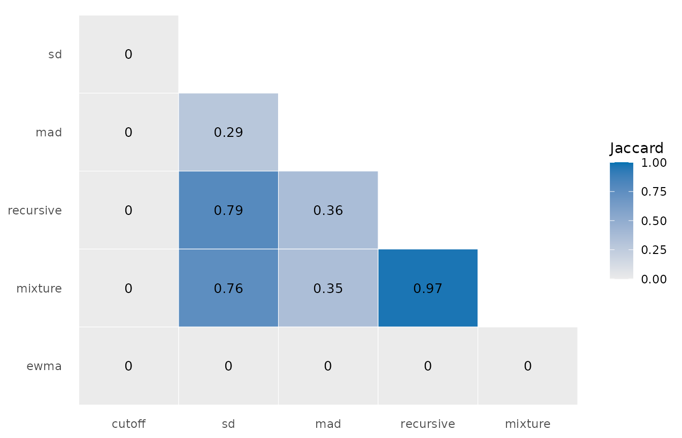

The threshold is part of the pipeline

policy and threshold are forwarded to every rule, and for the mixture they change what is removed. The same lognormal mixture at three thresholds:

vapply(c(0.3, 0.5, 0.7), function(th) {
  sum(!screen_compare(
    rt_example$rt, list(mixture = rule_mixture("lognormal")),
    .by = list(rt_example$id, rt_example$condition), threshold = th
  )$keep)
}, numeric(1)) |>
  setNames(c("0.3", "0.5", "0.7"))
#> 0.3 0.5 0.7 
#>  28  32  38

The deterministic rules are unaffected, because their .prob is 0 or 1 and every threshold strictly between falls on the same side.

With ground truth: score every rule at once

Everything above is available on real data. rt_example also carries the truth, and because keep is a matrix, scoring every rule is one line for sensitivity and one for specificity:

contaminant <- rt_example$contaminant

round(colMeans(!cmp$keep[contaminant, ]), 2)
#>    cutoff        sd       mad recursive   mixture      ewma 
#>      0.00      0.25      0.33      0.30      0.30      0.17
round(colMeans(cmp$keep[!contaminant, ]), 3)
#>    cutoff        sd       mad recursive   mixture      ewma 
#>     1.000     0.985     0.904     0.980     0.981     0.930

The most aggressive rule finds the most contaminants and pays the most genuine trials for them; the cutoff finds nothing because nothing in this fast task reaches its bounds. The ground-truth article shows the same scoring on data matched to your own task.

The roster as a table

The comparison object carries what it was given: cmp$rules holds the rule objects, each with its label, and a column mean of !cmp$keep is the realised drop rate per rule. Together they give one row per pipeline:

tibble(
  pipeline = names(cmp$rules),
  setting = vapply(cmp$rules, function(r) r$label, character(1)),
  prop_dropped = colMeans(!cmp$keep)
)
#> # A tibble: 6 × 3
#>   pipeline  setting              prop_dropped
#>   <chr>     <chr>                       <dbl>
#> 1 cutoff    cutoff(0.18, 3)            0     
#> 2 sd        sd(2.5, mean, sd)          0.0325
#> 3 mad       sd(2.5, median, mad)       0.114 
#> 4 recursive recursive(modified)        0.0412
#> 5 mixture   mixture(lognormal)         0.04  
#> 6 ewma      ewma(0.01, 1.5)            0.0775

Applying each column of keep to what comes next repeats the downstream analysis per pipeline: filter with a column, aggregate, estimate, and repeat. The aggregation article carries one such table through to drift estimates, and the ground-truth article adds the column a real data set never has, which is how far each pipeline sits from the truth.