Recovering between-subject correlations • bmmtools

A model that measures individual differences has to do more than order people correctly on each of its parameters. Most substantive questions are about how those differences relate: whether precision in one task goes with precision in another, whether two parameters of the same model are separable, or whether a parameter correlates with an ability measured outside the model. Validating a new bmm model scored how well subject estimates recover the subjects’ true values. This article scores how well the correlations between them are recovered.

A first look, not a benchmark. The results below come from one small simulation: four conditions, 20 replications each, 100 subjects per data set, fitted with four chains of 1,000 iterations, half of them warmup. At that length many fits miss the usual convergence standard, and we score them under a looser one (see Convergence). The results show how the tools work and in which direction each estimator errs. They are not a calibrated recommendation for study design. A more comprehensive simulation will replace this article once the package is stable.

To run the code you need bmm, brms, a working cmdstanr installation and, for the SEM part, lavaan. The output was computed once and saved, so this page was built without Stan or lavaan. Simulating and fitting the grid took 265 minutes.

Generating correlated people

library(bmmtools)

model <- bmm::mixture2p(resp_error = "y")
pars <- c(kappa = log(8), thetat = qlogis(0.75))
sds <- c(kappa = 0.3, thetat = 0.5)

The model is bmm’s two-parameter mixture model, with population values and between-subject SDs on the link scale as in Validating a new bmm model. Each simulated subject does two tasks with 100 trials each, so there are four subject-level terms, kappa and thetat in task 1 and task 2, and one observed covariate G, standing in for an ability measured by a separate test.

The correlations among these five variables come from a factor model:

loadings <- matrix(
  c(
    sqrt(0.7), sqrt(0.7), 0, 0, 0,
    0, 0, sqrt(0.7), sqrt(0.7), 0,
    0, 0, 0, 0, 1
  ),
  ncol = 3,
  dimnames = list(
    c("kappa_task1", "kappa_task2", "thetat_task1", "thetat_task2", "G"),
    c("precision", "memory", "ability")
  )
)
factor_cors <- function(rho) {
  phi <- matrix(rho, 3, 3, dimnames = rep(list(colnames(loadings)), 2))
  diag(phi) <- 1
  phi
}
cors_for <- function(row) cors_from_factors(loadings, factor_cors(row$rho))
round(cors_for(data.frame(rho = 0.5)), 2)
#>              kappa_task1 kappa_task2 thetat_task1 thetat_task2    G
#> kappa_task1         1.00        0.70         0.35         0.35 0.42
#> kappa_task2         0.70        1.00         0.35         0.35 0.42
#> thetat_task1        0.35        0.35         1.00         0.70 0.42
#> thetat_task2        0.35        0.35         0.70         1.00 0.42
#> G                   0.42        0.42         0.42         0.42 1.00

cors_from_factors() turns loadings and factor correlations into the implied correlation matrix. The two tasks load \(\sqrt{.7}\) on a factor per parameter, precision for kappa and memory for thetat, and G loads 1 on its own factor ability. All three factors correlate \(\rho\). This gives three kinds of pairs with known values:

the same parameter across tasks, \(.7\) at every \(\rho\);
different parameters, \(.7\rho\), so \(.35\) at \(\rho = .5\);
a parameter with G, \(\sqrt{.7}\,\rho\), so \(.42\) at \(\rho = .5\).

We used a factor model, rather than one correlation for every pair, for two reasons. First, the article can then separate the correlation between two terms, which the estimators below score, from the correlation between the latent factors, which a structural equation model recovers. Second, the factor model keeps that SEM identified even at \(\rho = 0\), because the two tasks of one parameter still correlate \(.7\).

Three estimators

extract_correlations() offers three answers to the question of how two subject-level terms correlate:

"model" is the correlation of the random effects the model estimates. It exists only when the random effects of the two terms share a correlation block, (1 | p | id).
"draws" correlates the subjects’ values within each posterior draw and summarises these correlations like any other posterior, with the median and a 95% equal-tailed credible interval (CrI).
"point" correlates the subjects’ posterior means, with a Fisher-z interval that treats the means as if they were observed values.

They target different quantities. model estimates the correlation in the population the subjects come from. draws describes the subjects in the data set: its interval reflects uncertainty about their values, not about which subjects happened to be sampled. point is a correlation of estimates, and so it inherits whatever shrinkage and estimation error those estimates carry. recover_correlations() therefore scores each estimate against two truths: true_value, the generating correlation, and sample_value, the correlation the simulated subjects actually had.

The grid

grid <- expand.grid(
  rho = c(0, 0.5),
  re_cor = c("none", "all"),
  stringsAsFactors = FALSE
)
grid$n_subjects <- 100
grid$n_trials <- 100
grid

The grid crosses the factor correlation, \(\rho = 0\) or \(.5\), with the random-effects structure of the fitted model. Under re_cor = "none" every term has its own random intercept and the model assumes the terms are uncorrelated. Under re_cor = "all" the four terms share one correlation block, so the model estimates their correlations.

out <- recovery_grid(
  model, grid, pars,
  dir = file.path(fits_dir, "correlation-recovery"),
  reps = 20,
  sds = sds, cors = cors_for,
  covariates = list(G = c(mean = 0, sd = 1)),
  tasks = c("1", "2"),
  formula = function(row) {
    recovery_formula(model, re_cor = row$re_cor, task_col = "task")
  },
  correlations = c("model", "draws", "point"),
  seed = 2026,
  chains = 4, iter = 1000, cores = 4, threads = brms::threading(3),
  backend = "cmdstanr", refresh = 0, silent = 2
)

cors and formula are functions of the grid row. cors_for() builds the correlation matrix for the row’s \(\rho\), and the formula function reads the row’s re_cor, which is how one grid compares two model specifications. tasks and covariates add the task dimension and G to the simulated data. correlations asks the grid to extract all three estimators from every fit; model rows exist only in the re_cor = "all" cells. threads enables within-chain parallelisation in brms; in a timing test with one 100-subject fit it cut the sampling time from 499 to 238 seconds.

Convergence

# The grid's own verdict uses check_convergence()'s defaults. At iter 1000
# many fits miss the usual bar (Rhat < 1.01, ESS > 400), mostly on the
# cor_ terms and a few of the 400 subject effects. The article scores the
# fits that pass the looser bar below and reports both verdicts.
bar <- list(rhat_max = 1.05, ess_bulk_min = 150, ess_tail_min = 150,
            divergent_max = 0)
strict_bar <- list(rhat_max = 1.01, ess_bulk_min = 400, ess_tail_min = 400,
                   divergent_max = 0)
convergence <- dplyr::bind_rows(lapply(seq_len(nrow(cells)), function(i) {
  fit <- readRDS(cells$file[[i]])
  verdict <- rlang::exec(check_convergence, fit, !!!bar)
  strict <- rlang::exec(check_convergence, fit, !!!strict_bar)
  tibble::tibble(
    condition = cells$condition[[i]],
    replication = cells$replication[[i]],
    verdict,
    pass_strict = strict$pass
  )
}))
kept <- convergence[convergence$pass, c("condition", "replication")]
dplyr::summarise(
  convergence,
  fits = dplyr::n(), pass = sum(pass), pass_strict = sum(pass_strict),
  .by = condition
)

#> # A tibble: 4 × 10
#>   condition   rho re_cor  fits  pass pass_strict max_rhat min_ess_bulk min_ess_tail
#>   <chr>     <dbl> <chr>  <int> <int>       <int>    <dbl>        <dbl>        <dbl>
#> 1 row-1       0   none      20    20           4     1.02         357.         626.
#> 2 row-2       0.5 none      20    20           2     1.02         338.         648.
#> 3 row-3       0   all       20    20           2     1.03         173.         333.
#> 4 row-4       0.5 all       20    20           4     1.02         244.         466.
#> # ℹ 1 more variable: n_divergent <int>

Under the usual standard, Rhat below 1.01, bulk and tail ESS above 400 and no divergent transitions, only 12 of the 80 fits pass. None had a divergent transition or hit the maximum tree depth; they fall short on Rhat and ESS, and not by much. The worst Rhat is 1.03, the smallest bulk ESS 173 and the smallest tail ESS 333. We therefore score every fit with Rhat below 1.05 and bulk and tail ESS above 150, which all 80 fits meet.

The shortfall is concentrated in a few variables:

# Where the fits miss the strict bar: per fit and group of variables, how
# many variables do.
variable_group <- function(variable) {
  dplyr::case_when(
    startsWith(variable, "b_") ~ "population",
    startsWith(variable, "sd_") ~ "sd",
    startsWith(variable, "cor_") ~ "cor",
    startsWith(variable, "r_") ~ "subject"
  )
}
convergence_groups <- dplyr::bind_rows(lapply(
  seq_len(nrow(cells)), function(i) {
    draws <- posterior::subset_draws(
      posterior::as_draws_df(readRDS(cells$file[[i]])),
      variable = "^(b|sd|cor|r)_", regex = TRUE
    )
    diag <- posterior::summarise_draws(draws, "rhat", "ess_bulk", "ess_tail")
    # a variable that is constant across draws has no rhat
    diag <- diag[!is.na(diag$rhat), ]
    diag$group <- variable_group(diag$variable)
    dplyr::summarise(
      diag,
      condition = cells$condition[[i]],
      replication = cells$replication[[i]],
      n_variables = dplyr::n(),
      n_rhat = sum(rhat >= strict_bar$rhat_max),
      n_ess = sum(ess_bulk <= strict_bar$ess_bulk_min |
                    ess_tail <= strict_bar$ess_tail_min),
      max_rhat = max(rhat),
      min_ess_bulk = min(ess_bulk),
      .by = group
    )
  }
))
dplyr::summarise(
  convergence_groups,
  fits_rhat = sum(n_rhat > 0), fits_ess = sum(n_ess > 0),
  max_rhat = max(max_rhat), min_ess_bulk = min(min_ess_bulk),
  .by = c(condition, group)
)

#> # A tibble: 7 × 7
#>   re_cor group       fits fits_rhat fits_ess max_rhat min_ess_bulk
#>   <chr>  <chr>      <int>     <int>    <int>    <dbl>        <dbl>
#> 1 none   population    40         6        1     1.02         398.
#> 2 none   sd            40         8        0     1.02         465.
#> 3 none   subject       40        26        0     1.01        1062.
#> 4 all    population    40         1        0     1.01         485.
#> 5 all    sd            40         0        0     1.01         551.
#> 6 all    cor           40        20       19     1.03         173.
#> 7 all    subject       40        13        0     1.01         416.

In the re_cor = "all" cells, 20 of 40 fits have a correlation parameter with Rhat of 1.01 or above, and 19 have one with ESS at or below 400. The smallest bulk ESS of any correlation parameter is 173. These are the draws the model estimator summarises, so its intervals below rest on fewer effective draws than the other estimators’. In the re_cor = "none" cells, 26 of 40 fits have at least one of their 400 subject-level terms with Rhat of 1.01 or above, 8 an SD and 6 a population parameter. Longer chains are the obvious remedy. For a simulation meant to show the direction of errors rather than exact calibration, we did not run them.

Scoring

design <- data.frame(condition = sprintf("row-%d", seq_len(nrow(grid))), grid)
cors_all <- attr(out, "correlations")
cors <- dplyr::semi_join(cors_all, kept, by = c("condition", "replication"))
cor_summary <- dplyr::left_join(summary(cors), design, by = "condition")
cor_summary

summary() of the correlation recovery has one row per condition, pair and estimator. With ten pairs, three estimators and four conditions this is a long table, so we average it within the three kinds of pairs:

pair_type <- function(term) {
  dplyr::case_when(
    grepl("(^|__)G(__|$)", term) ~ "with G",
    grepl("^kappa.*__kappa|^thetat.*__thetat", term) ~ "same parameter",
    TRUE ~ "across parameters"
  )
}
by_type <- res$cor_summary |>
  dplyr::mutate(pair_type = pair_type(term)) |>
  dplyr::summarise(
    true_value = mean(true_value),
    mean_estimate = mean(mean_estimate),
    bias = mean(bias),
    coverage = mean(coverage),
    coverage_sample = mean(coverage_sample),
    rejection_rate = mean(rejection_rate),
    ci_width = mean(ci_width),
    .by = c(pair_type, rho, re_cor, estimator)
  )
print(by_type, n = Inf)
#> # A tibble: 28 × 11
#>    pair_type           rho re_cor estimator true_value mean_estimate      bias coverage
#>    <chr>             <dbl> <chr>  <chr>          <dbl>         <dbl>     <dbl>    <dbl>
#>  1 same parameter      0   none   draws          0.7         0.325   -0.375       0    
#>  2 across parameters   0   none   draws          0           0.0321   0.0321      0.988
#>  3 with G              0   none   draws          0           0.00916  0.00916     0.762
#>  4 same parameter      0   none   point          0.7         0.476   -0.224       0.1  
#>  5 across parameters   0   none   point          0           0.104    0.104       0.888
#>  6 with G              0   none   point          0           0.0127   0.0127      0.962
#>  7 same parameter      0.5 none   draws          0.7         0.358   -0.342       0    
#>  8 across parameters   0.5 none   draws          0.35        0.183   -0.167       0.363
#>  9 with G              0.5 none   draws          0.418       0.315   -0.104       0.475
#> 10 same parameter      0.5 none   point          0.7         0.515   -0.185       0.175
#> 11 across parameters   0.5 none   point          0.35        0.318   -0.0316      0.925
#> 12 with G              0.5 none   point          0.418       0.377   -0.0409      0.888
#> 13 same parameter      0   all    model          0.7         0.662   -0.0381      0.975
#> 14 across parameters   0   all    model          0           0.00953  0.00953     0.975
#> 15 same parameter      0   all    draws          0.7         0.672   -0.0278      0.925
#> 16 across parameters   0   all    draws          0           0.00894  0.00894     0.925
#> 17 with G              0   all    draws          0          -0.0274  -0.0274      0.75 
#> 18 same parameter      0   all    point          0.7         0.798    0.0983      0.4  
#> 19 across parameters   0   all    point          0           0.0773   0.0773      0.75 
#> 20 with G              0   all    point          0          -0.0324  -0.0324      0.962
#> 21 same parameter      0.5 all    model          0.7         0.681   -0.0193      1    
#> 22 across parameters   0.5 all    model          0.35        0.330   -0.0195      0.962
#> 23 same parameter      0.5 all    draws          0.7         0.693   -0.00655     0.975
#> 24 across parameters   0.5 all    draws          0.35        0.349   -0.000929    0.85 
#> 25 with G              0.5 all    draws          0.418       0.365   -0.0530      0.675
#> 26 same parameter      0.5 all    point          0.7         0.825    0.125       0.35 
#> 27 across parameters   0.5 all    point          0.35        0.507    0.157       0.488
#> 28 with G              0.5 all    point          0.418       0.425    0.00628     0.962
#> # ℹ 3 more variables: coverage_sample <dbl>, rejection_rate <dbl>, ci_width <dbl>

rejection_rate is the share of replications whose interval excludes zero: the false-positive rate where the true correlation is 0 and the power where it is not. Recovery summary columns defines the other columns.

library(ggplot2)
ggplot(
  by_type,
  aes(estimator, mean_estimate, colour = re_cor)
) +
  geom_hline(aes(yintercept = true_value), linetype = "dashed") +
  geom_point(size = 2.5, position = position_dodge(width = 0.4)) +
  facet_grid(paste("rho =", rho) ~ pair_type) +
  labs(
    x = NULL, y = "Mean estimate (dashed: generating value)",
    colour = "re_cor"
  )

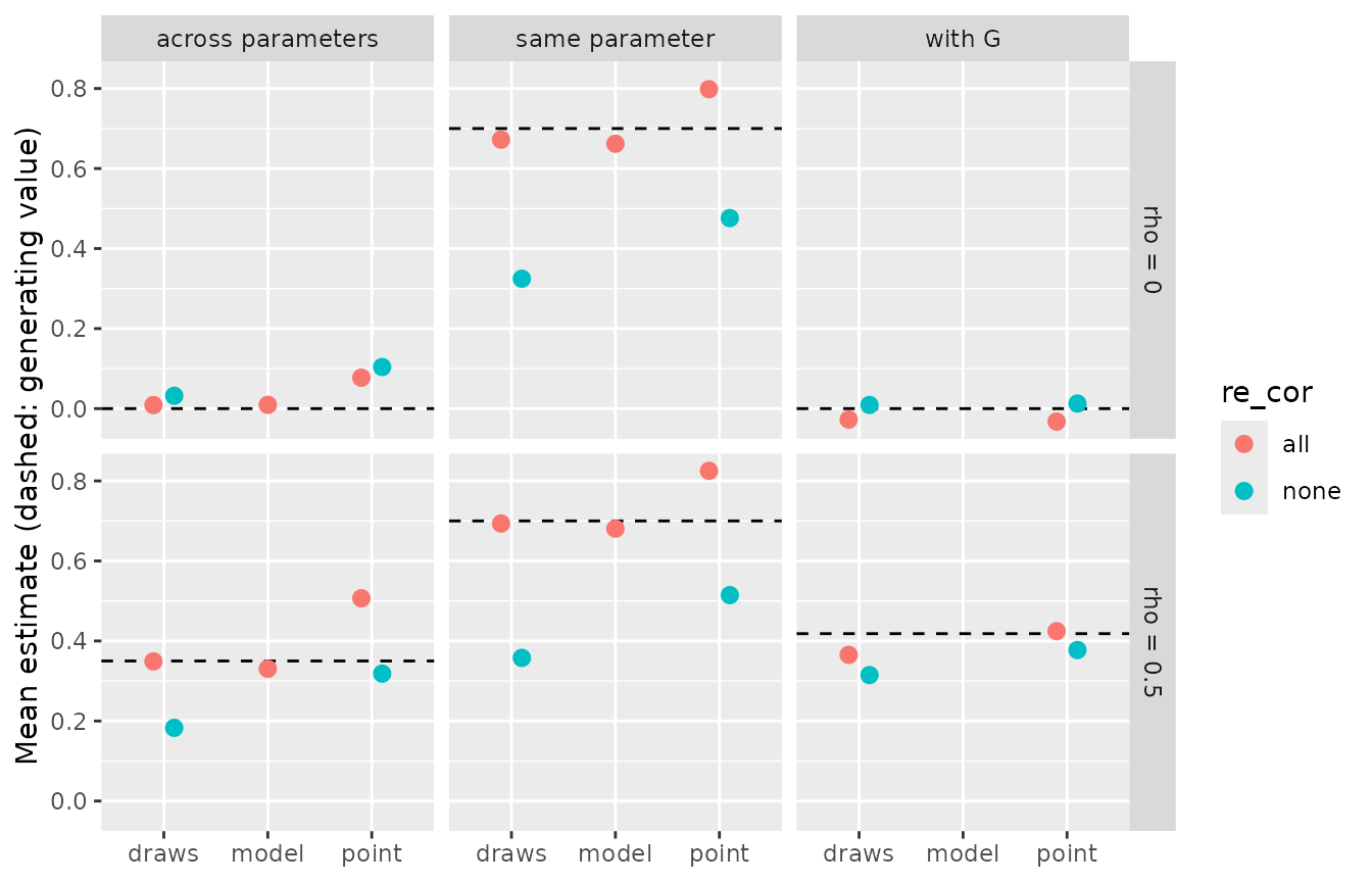
The same parameter across tasks. The generating correlation is .70. A model without correlated random effects shrinks each subject towards the mean of that term alone, and both estimators are attenuated: draws gives .36 and point .51 at \(\rho = .5\). With correlated random effects, model and draws recover the correlation, at .68 and .69. point now overshoots, at .83, and because its interval is narrow (mean width .13) it covers the generating value in only .35 of the replications. A likely reason is that the correlated model shrinks each subject towards the correlation it estimates, so the posterior means line up more closely than the true values do.

Different parameters. At \(\rho = 0\) this pair type measures false positives. Under re_cor = "all", point excludes zero in .25 of the replications, against .07 for draws and .02 for model. At \(\rho = .5\) (generating value .35) the same pattern holds: draws and model are close, .35 and .33, and point is inflated to .51. Under re_cor = "none", draws is attenuated to .18, while point lands near the truth at .32. However, the same point estimator gives .10 where the truth is 0, so this is not an unbiased estimator but, in this design, an attenuation and an upward bias that partly cancel.

A parameter with G. Here point is the best calibrated estimator. At \(\rho = 0\) it excludes zero in .04 of the replications under re_cor = "all", and at \(\rho = .5\) its mean is .42 against a generating value of .42, covered in .96 of the replications. draws excludes zero in .25 of the replications at \(\rho = 0\). This follows from its target: its interval covers the correlation these 100 subjects actually had in .97 of the replications. A sample of 100 subjects has a correlation with G that differs from 0 by chance, and the draws interval, which carries no uncertainty about which subjects were sampled, is narrow enough (mean width .21) to detect it.

Taken together, in this design, correlations between parameters of one model were best recovered by fitting correlated random effects and reading model or draws. Correlating posterior means from that model overstated the correlations and inflated false positives. For a correlation with an observed covariate, point answered the population question and draws the in-sample one.

plot_recovery() shows the replications of one cell, each estimate against the correlation the subjects actually had:

plot_recovery(dplyr::filter(cors, condition == "row-4"), truth = "sample") +
  ggplot2::theme(strip.text = ggplot2::element_text(size = 7))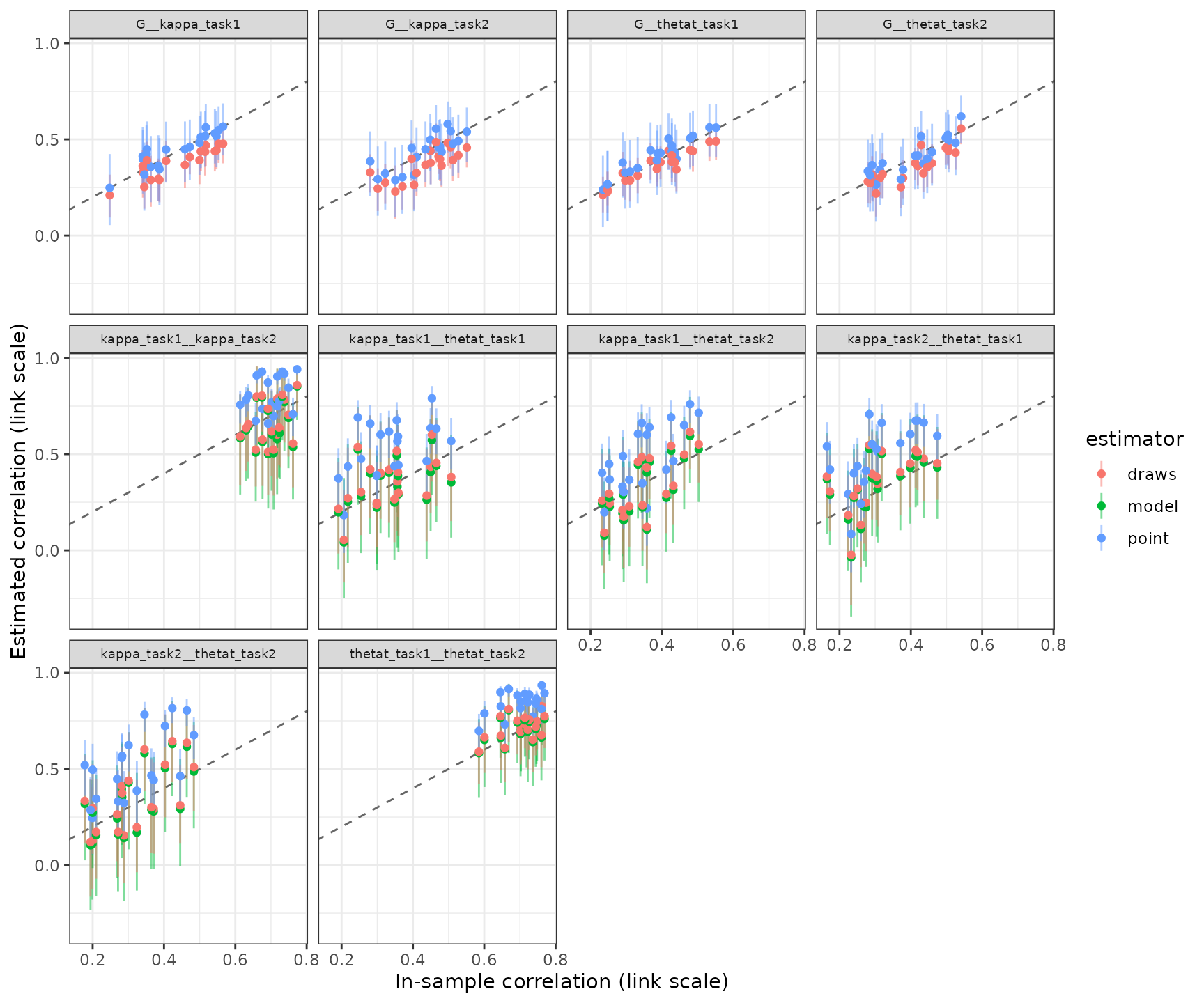

The SEM route

A second way to estimate a latent correlation is to take the subject estimates out of the model and fit a structural equation model to them. subject_table() returns one row per subject with the true and estimated value of every term and the covariates:

tab <- subject_table(out, point = "median")
tab <- dplyr::semi_join(tab, kept, by = c("condition", "replication"))
tab

stopifnot(requireNamespace("lavaan", quietly = TRUE))
# Two indicators per factor are identified only through the factor's
# correlations with the rest of the model, which vanish at rho = 0, so the
# two tasks share a loading: they are parallel by construction. kappa and
# thetat of one task are estimated from the same trials, so their
# estimation errors covary; the residual covariances take that up.
cfa_model <- "
  precision =~ l1 * est_kappa_task1 + l1 * est_kappa_task2
  memory    =~ l2 * est_thetat_task1 + l2 * est_thetat_task2
  est_kappa_task1 ~~ est_thetat_task1
  est_kappa_task2 ~~ est_thetat_task2
  precision ~~ memory + G
  memory    ~~ G
"
# Every fit is kept with its status: warnings are recorded, not dropped.
factor_correlations <- function(data, model, factors) {
  warnings <- character()
  fit <- withCallingHandlers(
    tryCatch(
      lavaan::cfa(model, data = data, std.lv = TRUE),
      error = function(e) e
    ),
    warning = function(w) {
      warnings <<- c(warnings, conditionMessage(w))
      invokeRestart("muffleWarning")
    }
  )
  status <- if (inherits(fit, "error")) {
    "error"
  } else if (!lavaan::lavInspect(fit, "converged")) {
    "not converged"
  } else if (length(warnings) > 0) {
    "warning"
  } else {
    "ok"
  }
  if (status %in% c("error", "not converged")) {
    return(data.frame(
      pair = NA_character_, estimate = NA_real_, ci_low = NA_real_,
      ci_high = NA_real_, status = status,
      message = paste(c(conditionMessage(fit)[inherits(fit, "error")],
                        warnings), collapse = " | ")
    ))
  }
  sol <- lavaan::standardizedSolution(fit)
  sol <- sol[sol$op == "~~" & sol$lhs %in% factors & sol$lhs != sol$rhs, ]
  data.frame(
    pair = paste(sol$lhs, sol$rhs, sep = "__"),
    estimate = sol$est.std,
    ci_low = sol$ci.lower,
    ci_high = sol$ci.upper,
    status = status,
    message = paste(unique(trimws(warnings)), collapse = " | ")
  )
}
lavaan_grid <- dplyr::bind_rows(
  lapply(split(tab, ~ condition + replication, drop = TRUE), function(d) {
    fc <- factor_correlations(d, cfa_model, c("precision", "memory"))
    cbind(d[1, c("condition", "replication")], fc, row.names = NULL)
  })
)
lavaan_grid <- dplyr::left_join(lavaan_grid, design, by = "condition")
lavaan_status <- dplyr::count(
  dplyr::distinct(lavaan_grid, condition, replication, status),
  condition, status
)
lavaan_grid_summary <- dplyr::summarise(
  dplyr::filter(lavaan_grid, !is.na(pair)),
  n_fits = dplyr::n(),
  n_warning = sum(status == "warning"),
  mean_estimate = mean(estimate),
  sd_estimate = stats::sd(estimate),
  # every latent correlation is rho: G loads 1 on its own factor
  coverage = mean(ci_low <= rho & ci_high >= rho),
  .by = c(condition, rho, re_cor, pair)
)
lavaan_status
lavaan_grid_summary

The CFA mirrors the generating model. Each parameter’s two tasks load on one factor with equal loadings, G is observed, and within a task the residuals of kappa and thetat covary, because both are estimated from the same trials. Every fit is kept with its status:

#>   condition  status  n
#> 1     row-1      ok 20
#> 2     row-2      ok 20
#> 3     row-3      ok  7
#> 4     row-3 warning 13
#> 5     row-4      ok  5
#> 6     row-4 warning 15
#>    condition rho re_cor              pair n_fits n_warning mean_estimate sd_estimate
#> 1      row-1 0.0   none precision__memory     20         0         0.248       0.132
#> 2      row-1 0.0   none      precision__G     20         0         0.050       0.157
#> 3      row-1 0.0   none         memory__G     20         0        -0.006       0.124
#> 4      row-2 0.5   none precision__memory     20         0         0.597       0.152
#> 5      row-2 0.5   none      precision__G     20         0         0.524       0.109
#> 6      row-2 0.5   none         memory__G     20         0         0.522       0.110
#> 7      row-3 0.0    all precision__memory     20        13         0.027       0.206
#> 8      row-3 0.0    all      precision__G     20        13        -0.037       0.069
#> 9      row-3 0.0    all         memory__G     20        13        -0.032       0.111
#> 10     row-4 0.5    all precision__memory     20        15         0.574       0.194
#> 11     row-4 0.5    all      precision__G     20        15         0.438       0.117
#> 12     row-4 0.5    all         memory__G     20        15         0.401       0.113
#>    coverage
#> 1      0.85
#> 2      0.90
#> 3      1.00
#> 4      0.85
#> 5      0.95
#> 6      0.85
#> 7      0.70
#> 8      1.00
#> 9      0.95
#> 10     0.45
#> 11     0.80
#> 12     0.70

Under re_cor = "none" all 40 CFAs fit without warnings. The correlations with G are recovered, at .52 and .52 for a latent .5, and .05 and -.01 for 0. The correlation between the two parameter factors is not: it is .25 where the factors are uncorrelated and .60 where they correlate .5. This is consistent with the upward bias of point between parameters seen above, which the CFA then corrects for attenuation and so enlarges.

Under re_cor = "all", 13 of 20 CFAs at \(\rho = 0\) and 15 of 20 at \(\rho = .5\) end with a warning: negative residual variances or a residual covariance matrix that is not positive definite. The factor correlation varies widely between replications, with an SD of .19 at \(\rho = .5\), and its 95% confidence interval covers .5 in .45 of them. One explanation, which this simulation does not test, is that posterior means from a model with correlated random effects already carry the correlation the model estimated, and a CFA on them has little room left to model it again.

In this design, the two-step route recovers correlations with an observed covariate but not the correlation between two parameters of the same model. lavaan ran in the precompute script; it is not a dependency of bmmtools.

Several models, separate fits

Sometimes the terms come from different models, fitted separately: precision in a visual working memory task and in a verbal one, each with its own bmm fit. recovery_component() describes one model, simulate_components() draws correlated subjects across several, and fit_components() fits each:

a <- recovery_component(model, pars, n_trials = 100, sds = sds, name = "a")
b <- recovery_component(model, pars, n_trials = 100, sds = sds, name = "b")
set_loadings <- loadings
rownames(set_loadings) <- c("a_kappa", "b_kappa", "a_thetat", "b_thetat", "G")
set <- simulate_components(
  list(a, b),
  n_subjects = 100,
  cors = cors_from_factors(set_loadings, factor_cors(0.5)),
  covariates = list(G = c(mean = 0, sd = 1)),
  seed = 2026
)
set$truth$cor

fits <- fit_components(
  set,
  dir = file.path(fits_dir, "correlation-recovery-components"),
  chains = 4, iter = 1000, cores = 4, threads = brms::threading(3),
  backend = "cmdstanr", refresh = 0, silent = 2
)
set_convergence <- dplyr::bind_rows(
  lapply(fits, function(fit) {
    verdict <- rlang::exec(check_convergence, fit, !!!bar)
    verdict$pass_strict <- rlang::exec(check_convergence, fit, !!!strict_bar)$pass
    verdict
  }),
  .id = "component"
)
set_convergence

#> # A tibble: 2 × 10
#>   component max_rhat min_ess_bulk min_ess_tail n_divergent n_max_treedepth n_variables
#>   <chr>        <dbl>        <dbl>        <dbl>       <int>           <int>       <int>
#> 1 a             1.01         543.         882.           0               0         206
#> 2 b             1.01         525.         980.           0               0         206
#> # ℹ 3 more variables: pass <lgl>, failed <chr>, pass_strict <lgl>

This example is a single data set of 100 subjects at \(\rho = .5\), so its numbers illustrate the arithmetic rather than estimate a bias. Both fits pass the looser bar; fit a misses the strict one on Rhat.

set_recovery <- recover_correlations(fits, set, estimator = c("draws", "point"))
set_summary <- summary(set_recovery)
set_summary

set_tab <- subject_table(set, fits)
terms <- c("a_kappa", "b_kappa", "a_thetat", "b_thetat")
reliability <- vapply(
  terms,
  function(term) {
    true <- set_tab[[paste0("true_", term)]]
    est <- set_tab[[paste0("est_", term)]]
    stats::cor(true, est)^2
  },
  numeric(1)
)
pairs <- c("a_kappa__b_kappa", "a_thetat__b_thetat")
attenuation <- set_summary[set_summary$term %in% pairs, ]
attenuation$rel_a <- reliability[sub("__.*", "", attenuation$term)]
attenuation$rel_b <- reliability[sub(".*__", "", attenuation$term)]
attenuation$expected <- ifelse(
  attenuation$estimator == "point",
  attenuation$true_value * sqrt(attenuation$rel_a * attenuation$rel_b),
  attenuation$true_value * attenuation$rel_a * attenuation$rel_b
)
attenuation$disattenuated <- attenuation$mean_estimate / ifelse(
  attenuation$estimator == "point",
  sqrt(attenuation$rel_a * attenuation$rel_b),
  attenuation$rel_a * attenuation$rel_b
)
attenuation[, c("term", "estimator", "true_value", "mean_estimate",
                "rel_a", "rel_b", "expected", "disattenuated")]

#> # A tibble: 4 × 8
#>   term               estimator true_value mean_estimate rel_a rel_b expected disattenuated
#>   <chr>              <chr>          <dbl>         <dbl> <dbl> <dbl>    <dbl>         <dbl>
#> 1 a_kappa__b_kappa   draws            0.7         0.265 0.671 0.584    0.274         0.675
#> 2 a_thetat__b_thetat draws            0.7         0.425 0.715 0.764    0.382         0.778
#> 3 a_kappa__b_kappa   point            0.7         0.402 0.671 0.584    0.438         0.642
#> 4 a_thetat__b_thetat point            0.7         0.612 0.715 0.764    0.517         0.827

Neither fit knows about the other model’s subjects, so a correlation across fits is attenuated by the reliabilities of the two subject estimates. Here the reliability is the squared correlation of true and estimated values, between .58 and .76. For kappa the generating correlation of .70 comes out as .40 with point and .26 with draws, close to the expected .44 for \(\rho\sqrt{rel_a\,rel_b}\) and .27 for \(\rho\,rel_a\,rel_b\). Dividing by those factors gives .64 and .67. For thetat both estimates lie above the expected values, .61 against .52 and .42 against .38, and their disattenuated values, .83 and .78, overshoot .70. A single data set cannot tell whether this is noise. In practice the reliabilities are not known and would have to be estimated as well.

# Within each model, kappa and thetat come from the same fit and trials,
# so their estimation errors covary.
cfa_set <- "
  precision =~ est_a_kappa + est_b_kappa
  memory    =~ est_a_thetat + est_b_thetat
  est_a_kappa ~~ est_a_thetat
  est_b_kappa ~~ est_b_thetat
  precision ~~ memory + G
  memory    ~~ G
"
lavaan_set <- factor_correlations(set_tab, cfa_set, c("precision", "memory"))
lavaan_set

#>                pair estimate ci_low ci_high status
#> 1 precision__memory    0.806  0.578   1.035     ok
#> 2      precision__G    0.546  0.333   0.759     ok
#> 3         memory__G    0.390  0.194   0.586     ok

The CFA on the separate fits recovers the correlations with G, .55 and .39, and overestimates the correlation of the two parameter factors at .81, the same direction as in the grid. A joint multivariate fit of both models would estimate these correlations directly; bmmtools does not support that yet.

Which function does what

Step	Function	Returns
truth	`cors_from_factors()`	a correlation matrix implied by a factor model
simulate	`simulate_recovery()`, `simulate_components()`	data and truth, with tasks and covariates
formula	`recovery_formula(re_cor = )`	random intercepts, correlated or not
fit	`fit_cached()`, `fit_components()`	fits, reused while nothing changed
gate	`check_convergence()`	diagnostics and a verdict under your thresholds
extract	`extract_correlations()`	`model`, `draws` and `point` correlations
score	`recover_correlations()`	estimates against true and sample correlations
summarise	`summary()`	one row per pair, estimator and condition
two-step	`subject_table()`	true and estimated values per subject, for an SEM
loop	`recovery_grid(correlations = )`	all of the above over a design grid