Prior predictive checks on the observable scale • bmmtools

Priors of cognitive measurement models are set on the link scale, and what a normal(0, 1) there means for the data is rarely obvious. prior_check() answers that directly: it fits the model with sample_prior = "only", draws from the prior predictive distribution and summarises the draws on the scale of the response. Because the draws come from bmm’s own fit, the prior being checked is exactly the prior bmm fits with, defaults included.

The fits go through fit_cached(), so each prior set compiles and samples once and later calls reuse it. Two checks are shown below: a signal detection model, whose count response has a floor and a ceiling, and a mixture model with a statistic of our own.

A count response: sdt_yn

The first example is the check behind prior_check_sdt_yn, the prior check that ships with the package. It compares bmm’s default priors with a set that narrows the priors on the between-subject SDs:

sdt <- bmm::sdt_yn(response = "hits", stimulus = "stim", n_trials = "n")
sdt_data <- simulate_recovery(
  sdt,
  pars = c(d = 1, criterion = 0.3), sds = c(d = 0.3, criterion = 0.3),
  n_subjects = 20, n_trials = 50, seed = 2026
)$data

narrow_sd <- brms::set_prior("normal(0, 1)", class = "sd", dpar = "d") +
  brms::set_prior("normal(0, 1)", class = "sd", dpar = "criterion")

prior_check_sdt_yn <- prior_check(
  sdt, recovery_formula(sdt), sdt_data,
  prior = list(default = NULL, narrow_sd = narrow_sd),
  n_draws = 100, seed = 2026,
  file = "data-raw/fits/prior-check/sdt_yn",
  chains = 2, iter = 1000, backend = "cmdstanr", refresh = 0, silent = 2
)

prior is either one prior (or NULL for bmm’s defaults) or a named list of prior sets. Each set is fitted separately, its fit cached at <file>-<set>, and becomes one level of the prior column.

prior_check_sdt_yn
#> <bmmtools_prior_check>
#> Model: Signal Detection Theory (Yes/No); 2 prior sets: default, narrow_sd.
#> Prior-predictive draws per set: 100.
#> 
#> # A tibble: 5 × 5
#>   response statistic    default narrow_sd difference
#>   <chr>    <chr>          <dbl>     <dbl>      <dbl>
#> 1 hits     floor_rate     0.392     0.152     -0.241
#> 2 hits     ceiling_rate   0.420     0.146     -0.274
#> 3 hits     q50           30        23         -7    
#> 4 hits     q90           50        50          0    
#> 5 hits     q95           50        50          0

The default summary has five statistics per response:

floor_rate and ceiling_rate: the share of all prior-predictive values, over draws and observations, at or below the floor and at or above the ceiling of the response;
q50, q90 and q95: quantiles of the prior-predictive values.

For sdt_yn and sdt_mafc the floor is 0 and the ceiling is the trial count of each row, read from the model’s n_trials column. With exactly two prior sets, summary() adds a difference column, the second set minus the first. Here, 39.2% of the prior-predictive counts under bmm’s defaults are at 0 and 41.9% at the ceiling; with the narrower SD priors the shares are 15.2% and 14.6%.

summary(prior_check_sdt_yn)
#> # A tibble: 5 × 5
#>   response statistic    default narrow_sd difference
#>   <chr>    <chr>          <dbl>     <dbl>      <dbl>
#> 1 hits     floor_rate     0.392     0.152     -0.241
#> 2 hits     ceiling_rate   0.420     0.146     -0.274
#> 3 hits     q50           30        23         -7    
#> 4 hits     q90           50        50          0    
#> 5 hits     q95           50        50          0

For a discrete response, plot the draws as histograms:

plot_prior_check(prior_check_sdt_yn, type = "histogram")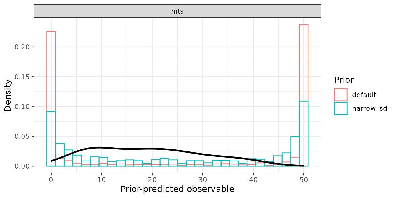

type = "statistic" plots the summary table instead, one point per statistic and prior set:

plot_prior_check(prior_check_sdt_yn, type = "statistic")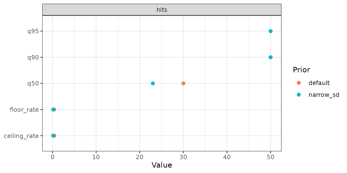

A continuous response and a statistic of your own

For a continuous response, a value exactly at a bound has probability zero, so the two rates are only informative for counts. For the circular models mixture2p and sdm the range is set to -pi and pi, and the rates report mass outside it. The quantiles of a signed circular error are symmetric about zero, so a statistic on the absolute error says more. summary takes any function of yrep, the matrix of prior-predictive draws (draws in rows, observations in columns), and data, and returns a data frame with the columns statistic and value, plus response for a model with several responses:

mix <- bmm::mixture2p(resp_error = "y")
mix_data <- simulate_recovery(
  mix,
  pars = c(kappa = log(8), thetat = qlogis(0.75)),
  sds = c(kappa = 0.3, thetat = 0.5),
  n_subjects = 10, n_trials = 40, seed = 1
)$data

abs_error <- function(yrep, data) {
  tibble::tibble(
    statistic = c("abs_q50", "abs_q90"),
    value = unname(stats::quantile(abs(yrep), c(0.5, 0.9)))
  )
}
mix_check <- prior_check(
  mix, recovery_formula(mix), mix_data,
  summary = abs_error,
  n_draws = 50, seed = 1,
  file = file.path(fits_dir, "prior-mixture2p"),
  chains = 2, iter = 1000, backend = "cmdstanr"
)
summary(mix_check)

#> # A tibble: 2 × 3
#>   response statistic default
#>   <chr>    <chr>       <dbl>
#> 1 y        abs_q50     0.734
#> 2 y        abs_q90     2.64

The default plot draws one thin density line per prior-predictive draw, so the spread between draws stays visible, with the observed response from data on top:

plot_prior_check(mix_check, draws = 30)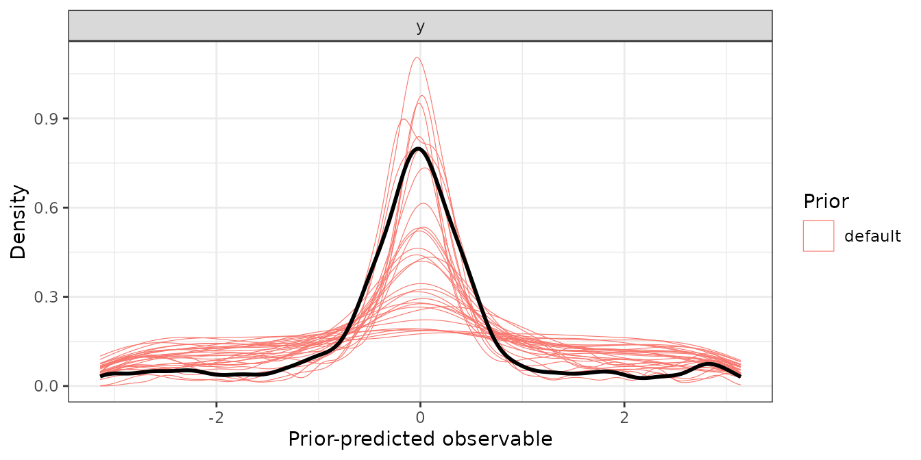

observed = FALSE removes the overlay. It is left out without comment when data has no response column, for example when the check runs over a design skeleton rather than simulated or real data.

Arguments worth knowing

range: The floor and the ceiling of the response as two numbers. NULL derives them for sdt_yn, sdt_mafc, mixture2p and sdm; for any other model the two rates are NA and a message says so.
n_draws: Prior-predictive draws kept per prior set. Asking for more than the fit holds is capped with a message rather than refused.
seed: Passed to the fitter, where it enters the cache key, and used around the draw subsample, so the same seed keeps the same draws.
file: Where the prior-only fits are cached. NULL uses a temporary file, so the compiled model is reused within the session and nothing is left on disk.
...: Passed to fit_cached() and on to bmm::bmm(): chains, iter, backend, cores. Giving sample_prior is an error, because the check sets it.

A population-level slope without a proper prior triggers a warning before fitting, because prior-only sampling has nothing to draw a flat prior from. bmm’s defaults cover the intercepts and the group-level SDs, so the warning concerns slopes you added to the formula.

What the object carries

Besides the summary rows, a bmmtools_prior_check keeps the draws, the brms::prior_summary() of each fit, the data, the model, the formula and the cache files as attributes. The prior summary records the prior that produced the draws, which is the one to report:

attr(prior_check_sdt_yn, "priors")$narrow_sd
#>            prior     class      coef group resp      dpar nlpar lb ub tag  source
#> 1 normal(0, 1.5) Intercept                      criterion                    user
#> 2   normal(1, 1) Intercept                              d                    user
#> 3    constant(0) Intercept                        sdratio                    user
#> 4   normal(0, 1)        sd                      criterion        0           user
#> 5   normal(0, 1)        sd                              d        0           user
#> 6                       sd              id      criterion                 default
#> 7                       sd Intercept    id      criterion                 default
#> 8                       sd              id              d                 default
#> 9                       sd Intercept    id              d                 default