Recovering the EZ diffusion model on the standard grid

This page reports one parameter recovery study of the three-parameter EZ diffusion model, bmm::ezdm(), fitted with bmm 1.4.1. The model describes each person’s accuracy and response times by a drift rate (drift), a boundary separation (bound) and a non-decision time (ndt), estimated in one Bayesian hierarchical model. Data were simulated from known parameter values, the model was fitted to them, and the estimates were compared with the values that generated the data. A researcher planning an EZ diffusion study can read from it how well each parameter is recovered with 20 or 50 subjects and 30, 100 or 300 trials per subject, and how many trials per person an analysis of individual differences needs at the generating values used here. It does not say how many subjects a study of group means or of correlations between parameters needs; it shows only what 20 and 50 subjects give.

A design is one combination of subjects and trials; the grid has six. Each design was simulated and fitted 10 times, the replications, so the study has 60 fits. The page reads every number from the stored results of those fits, so the page builds without refitting anything. bmmtools plans a validation card for each model it supports, a standard report on the same grid of designs; the card for ezdm will replace this page (issue #21).

Reading the figures. Most figures below are drawn by plot_design(): a quantity on the y axis, the number of trials on a log x axis, one line for 20 and one for 50 subjects, and one panel per parameter. Each row of panels has its own y axis, shared by the panels in it. A point is the mean over a design’s ten replications, and its bar shows how precisely ten replications pin that mean down. For bias and interval width the bar is ±1 Monte Carlo standard error (MCSE), the SD over the replications divided by √10; for RMSE it is ±1 MCSE of the mean squared error, divided by twice the RMSE (the delta method). For coverage and other shares the bar is a 95 % Wilson interval: the range of true shares that the observed count is consistent with. It stays between 0 and 1 and is not empty at 10 of 10: ten covered intervals out of ten are consistent with a true coverage as low as 0.723, the lower end of the bar. A dashed line marks the target where there is one: zero for bias, the nominal 0.95 for coverage. The help page of plot_design() states the source of every bar. The numbers behind each figure are in a table under it, folded away; the text does not need them.

The model and the generating values

The values below are on each parameter’s link scale, explained after the code.

library(bmmtools)

model <- bmm::ezdm(
  mean_rt = "mean_rt", var_rt = "var_rt", n_upper = "n_upper",
  n_trials = "n_trials"
)
# population means on each parameter's link scale: drift rate 1.5
# (identity link), boundary separation exp(0) = 1 (log link),
# non-decision time 0.3 s (log link)
pars <- c(drift = 1.5, bound = 0, ndt = log(0.3))
# between-subject SDs of the person-level values, on the same scales
sds <- c(drift = 0.3, bound = 0.2, ndt = 0.2)
# between-subject correlations: people who drift faster also set wider
# boundaries (0.4); the other two pairs are uncorrelated
cors <- diag(3)
dimnames(cors) <- rep(list(names(pars)), 2)
cors["drift", "bound"] <- cors["bound", "drift"] <- 0.4

# The prior SD of each parameter under bmm's default priors, in closed
# form, for the contraction column: normal(., 0.5) on the bound and ndt
# intercepts, exponential(1) on sd(drift) and exponential(2) on the other
# two SDs. drift's intercept prior is cauchy(0, 1), which has no SD, so it
# has no row and its contraction is NA.
prior_sd <- data.frame(
  term = c("bound", "ndt", "drift", "bound", "ndt"),
  level = c("population", "population", "sd", "sd", "sd"),
  prior_sd_link = c(0.5, 0.5, 1, 0.5, 0.5)
)

Each parameter is estimated on its link scale, the unbounded scale the model works on: drift as it is, bound and ndt as logarithms, so a between-subject SD of 0.2 on ndt means people differ by about 20 % in non-decision time. The three-parameter EZ model fixes s, the within-trial noise of the diffusion process, to 1. At these population values a person answers correctly on 81.8 % of trials, with a mean response time of 0.51 s (the EZ expressions for accuracy and mean response time with s = 1). prior_sd holds the prior SD of each parameter under bmm’s default priors; it is used for the contraction reported in the tables.

The run

out <- recovery_grid(
  model,
  grid = expand.grid(n_subjects = c(20, 50), n_trials = c(30, 100, 300)),
  pars = pars, sds = sds, cors = cors,
  dir = file.path(fits_dir, "recovery-ezdm"),
  reps = 10,
  re_cor = "all",
  levels = c("population", "sd", "subject"),
  correlations = "model",
  prior_sd = prior_sd,
  seed = 3131,
  chains = 4, iter = 2000, warmup = 1000, cores = 4,
  backend = "cmdstanr", refresh = 0, silent = 2
)

reps = 10 is the number of replications per design. bmmtools 0.2.0, which ran the script, did not pass seed on to the chains’ starting values, so a second run gave estimates that differ in the third decimal; later versions seed them too. The one place where that matters is said below.

What the other arguments do

re_cor = "all" lets the model estimate all three between-subject correlations. levels and correlations = "model" choose what is compared with the truth: the population means, the between-subject SDs, every subject’s parameters, and the model’s correlation estimates. seed fixes the simulated data and the sampler’s seed. The arguments after it go to bmm::bmm(): four chains of 2000 iterations each, the first 1000 of them warm-up. The help page of recovery_grid() explains the rest.

plot_design(out, type = "convergence")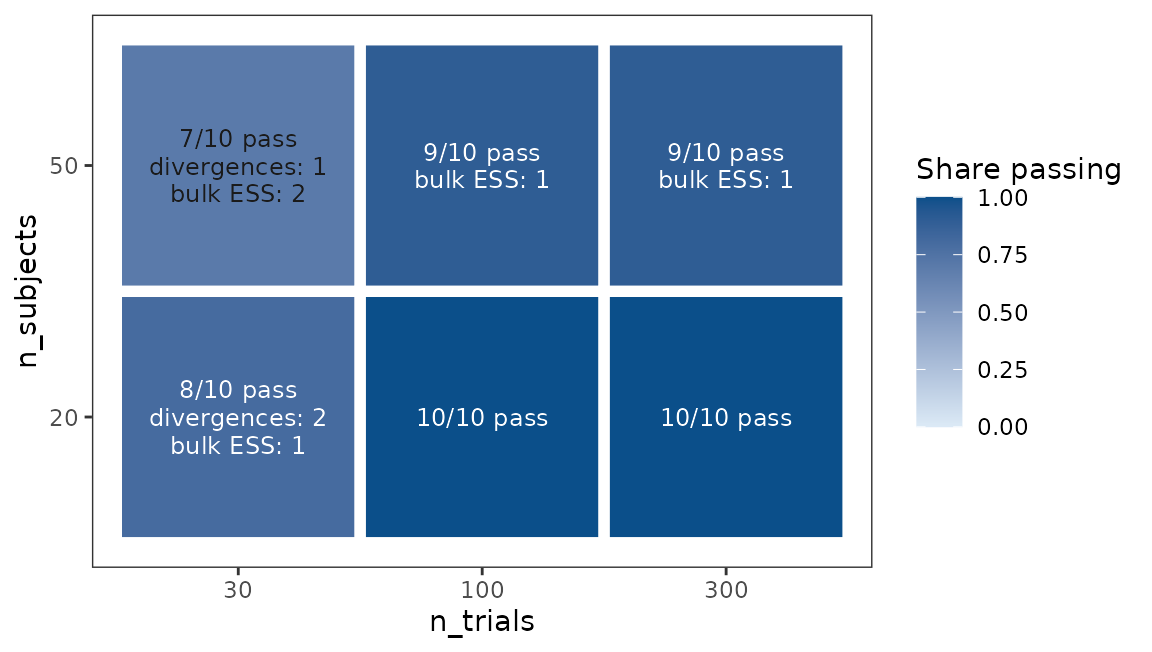

Every fit goes through bmmtools’ convergence gate, which asks whether the sampler explored the posterior well enough to trust the fit. A tile counts the fits that fail each check, and one fit can fail more than one.

What the gate checks

The gate checks every parameter of the fit, the between-subject correlations and each person’s values included, and also lp__ and lprior, the log posterior and the log prior. R-hat compares the chains and should be close to 1; the gate allows at most 1.05. The effective sample size (ESS) counts how many independent draws the chains are worth; the gate asks for at least 400 in the bulk of the posterior. The ESS in its tails is reported, not gated. Divergent transitions are steps where the sampler failed; the gate allows at most 10.

53 of the 60 fits pass; 46 pass if R-hat must also be at most 1.01. Of the 7 fits that fail, 5 are at 30 trials; 5 fail on bulk ESS and 3 on divergences. Leaving out lp__ and lprior, the lowest bulk ESS sits on a between-subject correlation in most fits, failing or not (6 of 7, and 46 of the 53 that pass), and on a population mean in none that fails and in 5 of those that pass. The results below use every fit; using only those that pass changes no r_low value (the lower end of the interval of r, defined with the subject parameters) by more than 0.033.

plot_design(out, metric = "fit_seconds")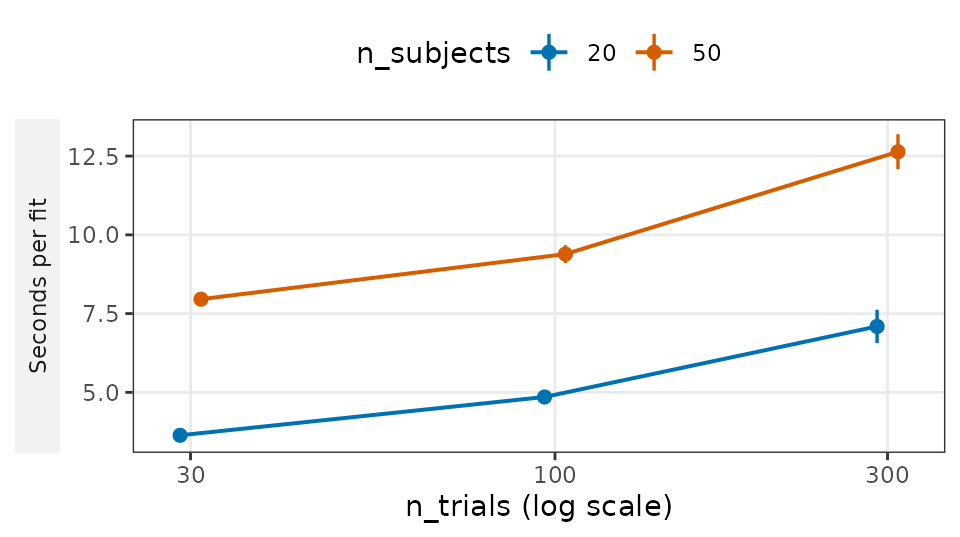

A point is the mean seconds per fit of a design. Fitting took 7.6 minutes in all (bmm 1.4.1, CmdStan 2.40.0), between 3.3 and 14.4 seconds per fit.

The convergence numbers per design

subjects	trials	fits passing the gate	passing with R-hat ≤ 1.01	fits with any divergence (the gate allows 10)	mean seconds per fit
20	30	8	7	8	3.6
20	100	10	10	3	4.9
20	300	10	10	4	7.1
50	30	7	5	5	8.0
50	100	9	7	0	9.4
50	300	9	7	0	12.6

Population means

plot_design(out)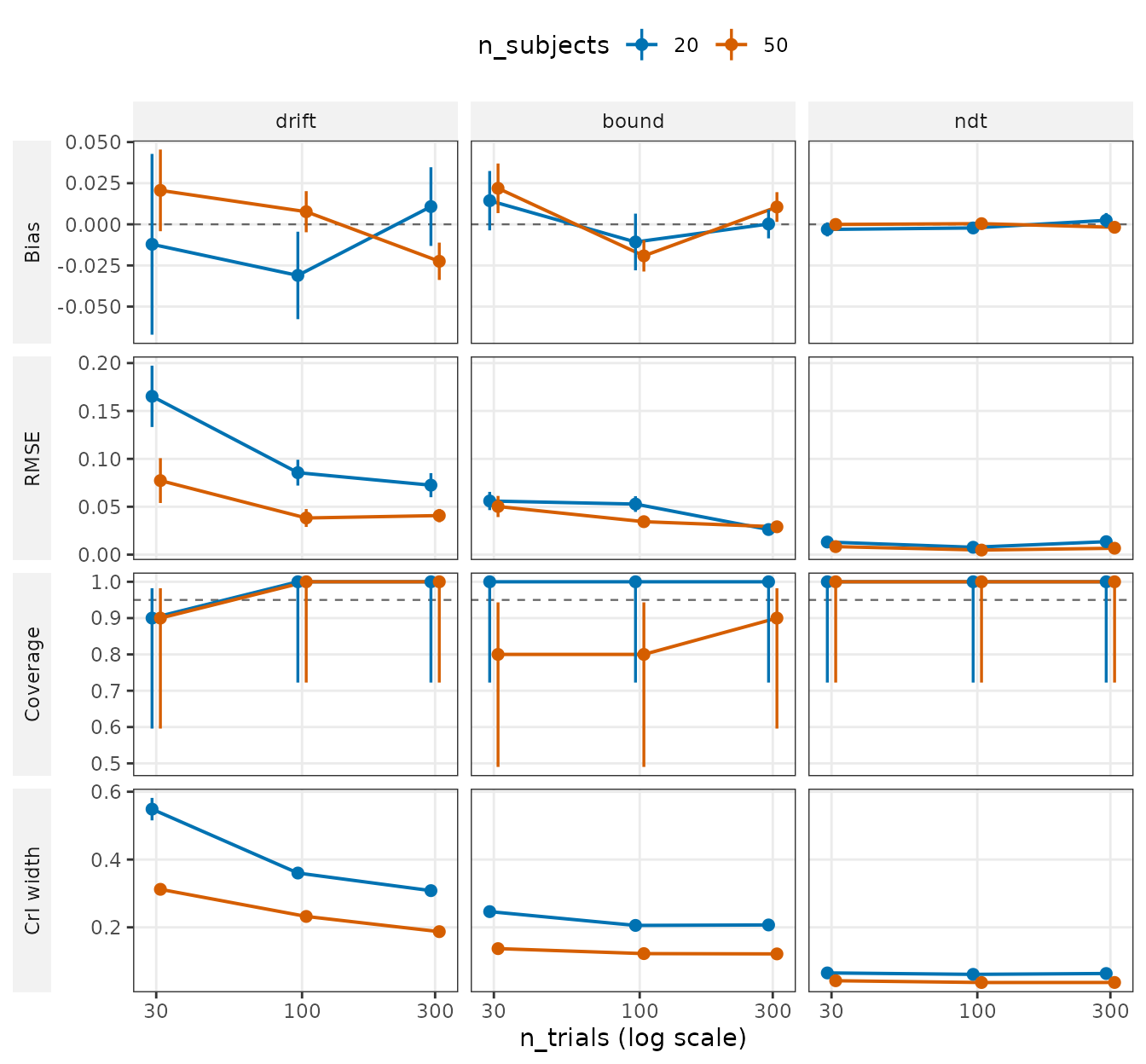

For each fit the estimate is the posterior median. Bias is the mean, over the ten replications, of estimate minus generating value; RMSE is the root of the mean squared difference; CrI width is the mean width of the 95 % credible interval (CrI); all three are on the natural scale, seconds for ndt. Because ndt is in seconds, its panels in these three rows look flat on the y axis each row shares; do not compare them with drift’s by height. Coverage is the share of the replications whose 95 % CrI contains the generating value. Intervals of the right width contain it 95 % of the time; intervals that contain it less often are too narrow, and ones that contain it more often are too wide. For a Bayesian interval at fixed generating values this holds only approximately (exactly only on average over the prior); the approximation is close here because the data outweigh the prior, with a mean contraction of at least 0.97 in the tables below and, for drift’s population mean, which has none, a posterior SD of at most 0.18 against the Cauchy prior’s scale of 1.

The population means show no bias of practical size: at most 0.032 in absolute value, and at most 2.2 % of the generating value. In 5 of the 18 cells the ±1 MCSE bar misses zero; with no bias at all, 6.2 would on average if the estimates are normal around the truth. More subjects narrow the intervals at every design and, for drift, lower the RMSE. Coverage is where ten replications show their limit. The CrI of bound covered in 8 of 10 replications with 50 subjects at both 30 and 100 trials. The Wilson interval of 8 of 10 runs from 0.49 to 0.94, ending just below 0.95. Across the 18 cells that is no more than chance gives: intervals of the right width cover in 8 or fewer of 10 with probability 0.086, so 1.55 of the 18 cells are expected to cover that rarely, and this run has 2. Pooled over all six designs, bound’s intervals cover at a rate whose interval contains 0.95 (the pooled coverage figure below).

plot_design(out, type = "coverage")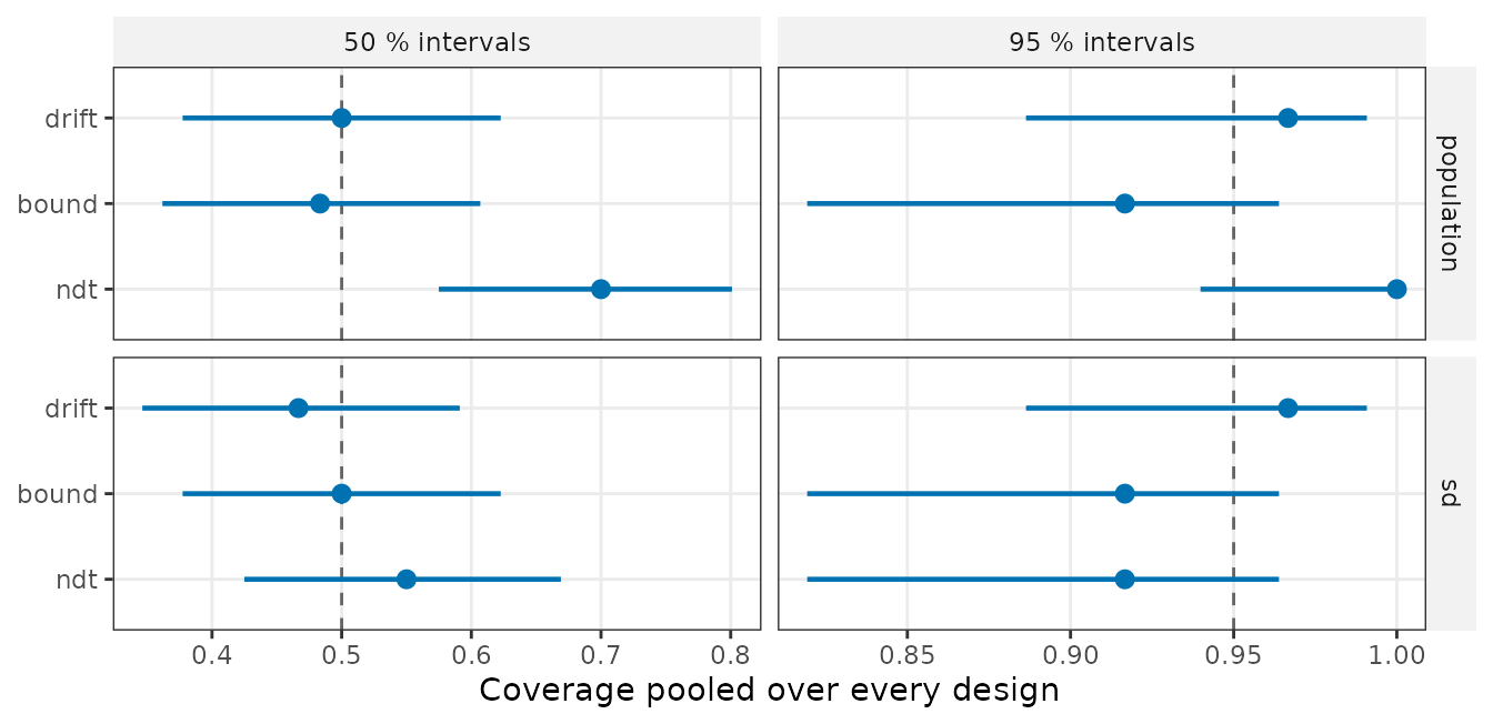

This figure pools the six designs, so each parameter has 60 intervals, on the assumption that all six share one coverage. Besides the 95 % interval, every fit also reported a 50 % interval, a second check of the width: it should contain the truth half of the time. Population means are in the upper row, between-subject SDs in the lower. For the 95 % intervals, 60 are still few: their Wilson interval excludes 0.95 only at 53 or fewer covered, which a true coverage of 0.90 gives with probability 0.39 and one of 0.85 with 0.82. Even at 60 of 60 it reaches down to 0.940, so it cannot show intervals that are too wide.

Every pooled Wilson interval contains its nominal value but one: population ndt’s 50 % intervals cover in 42 of 60 (Wilson interval 0.57 to 0.80, which excludes 0.50). With 12 intervals in the figure, one such miss is no surprise: if each missed by chance one time in 20, independently, at least one would with probability 0.46. But the exact binomial p-value of 42 of 60 at 0.50 is 0.0027, below 0.05 / 12 = 0.0042. The 95 % intervals of population ndt cover in all 60; they come from the same posteriors, so they are not a second finding. Its 50 % intervals are wider than their nominal mass. This run is the only evidence for it so far: the second run mentioned above used the same simulated data, so it cannot confirm it.

The population numbers per design

Contraction is 1 − (posterior SD / prior SD)², both on the link scale, unlike the other columns: near 1 when the data determine the estimate and near 0 when the posterior is still the prior. Averaged over the replications, as in the table, it is at least 0.984 for bound and ndt: a posterior variance, on average, at most 1.6 % of the prior variance. drift has none, because its default prior on the population value is a Cauchy distribution, which has no SD.

subjects	trials	parameter	bias	RMSE	covered	CrI width	contraction
20	30	drift	-0.012	0.165	9/10	0.549	–
20	30	bound	0.014	0.056	10/10	0.246	0.985
20	30	ndt	-0.003	0.013	10/10	0.065	0.987
20	100	drift	-0.031	0.086	10/10	0.360	–
20	100	bound	-0.011	0.053	10/10	0.206	0.989
20	100	ndt	-0.002	0.008	10/10	0.061	0.989
20	300	drift	0.011	0.073	10/10	0.308	–
20	300	bound	0.000	0.026	10/10	0.207	0.989
20	300	ndt	0.002	0.014	10/10	0.064	0.988
50	30	drift	0.021	0.077	9/10	0.312	–
50	30	bound	0.022	0.050	8/10	0.137	0.995
50	30	ndt	-0.000	0.008	10/10	0.042	0.995
50	100	drift	0.008	0.038	10/10	0.232	–
50	100	bound	-0.019	0.034	8/10	0.122	0.996
50	100	ndt	0.000	0.005	10/10	0.037	0.996
50	300	drift	-0.022	0.041	10/10	0.187	–
50	300	bound	0.011	0.029	9/10	0.122	0.996
50	300	ndt	-0.002	0.007	10/10	0.037	0.996

Between-subject SDs

plot_design(out, level = "sd")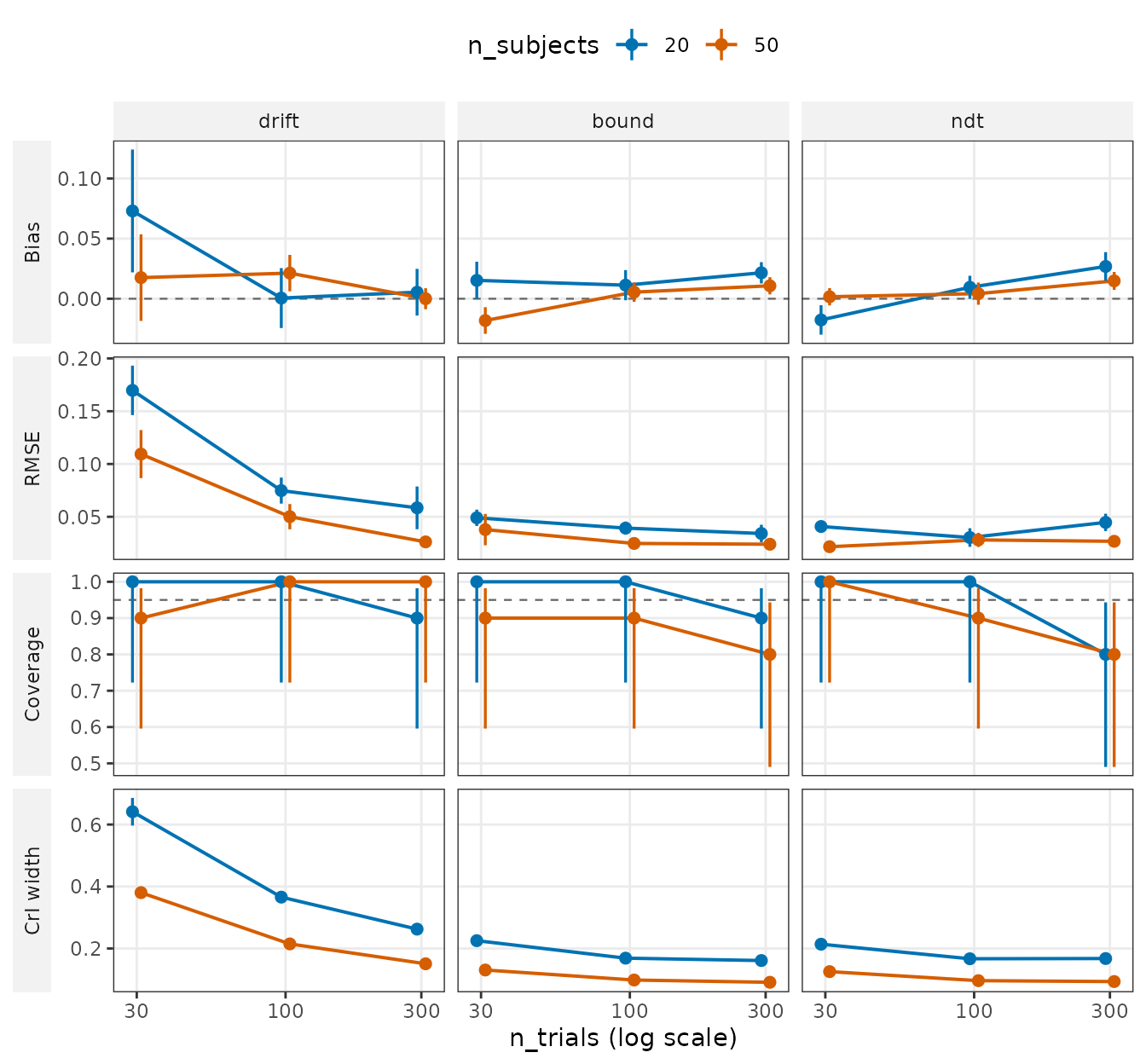

The SDs are read the same way, but on the link scale. Their bias is at most 0.073, for drift at 20 subjects and 30 trials. Their coverage drops to 8/10 at 300 trials (bound with 50 subjects, ndt with 20 subjects, ndt with 50 subjects), with the same wide Wilson interval as above; pooled over the designs, every SD’s interval contains the nominal rate (the figure above). Over the three SDs and both numbers of subjects, 52 of 60 intervals cover at 300 trials, against 58 at 30 and at 100, and all 8 that miss at 300 lie above the truth, their lower ends by at most 0.029. If misses fell above and below equally often, all 8 would fall on one side with probability 0.0078. That treats the misses as independent, but two of them come from one fit; counting the 7 fits instead gives 2 × 0.5⁷ = 0.016. This was found by looking at the results, not tested in advance. It fits a small positive bias: the mean bias of the SDs is 0.012, 0.009 and 0.013 at 30, 100 and 300 trials, and zero or above in all 12 cells from 100 trials on. Relative to the interval width, the bias is larger at 300 trials than at 100 in all 5 cells with a miss at 300. Ten replications cannot settle this, and the pooled figure, which assumes one coverage for all six designs, cannot show it.

The SD numbers per design

subjects	trials	parameter	bias	RMSE	covered	CrI width	contraction
20	30	drift	0.073	0.170	10/10	0.641	0.973
20	30	bound	0.015	0.049	10/10	0.225	0.987
20	30	ndt	-0.018	0.041	10/10	0.214	0.988
20	100	drift	0.001	0.075	10/10	0.366	0.991
20	100	bound	0.011	0.039	10/10	0.169	0.992
20	100	ndt	0.009	0.030	10/10	0.167	0.993
20	300	drift	0.005	0.058	9/10	0.262	0.995
20	300	bound	0.022	0.034	9/10	0.161	0.993
20	300	ndt	0.027	0.045	8/10	0.168	0.992
50	30	drift	0.018	0.109	9/10	0.380	0.990
50	30	bound	-0.018	0.038	9/10	0.131	0.996
50	30	ndt	0.002	0.022	10/10	0.125	0.996
50	100	drift	0.021	0.050	10/10	0.215	0.997
50	100	bound	0.005	0.025	9/10	0.098	0.997
50	100	ndt	0.004	0.028	9/10	0.096	0.998
50	300	drift	0.000	0.026	10/10	0.151	0.999
50	300	bound	0.011	0.024	8/10	0.091	0.998
50	300	ndt	0.015	0.027	8/10	0.093	0.998

Subject parameters

plot_design(out, level = "subject")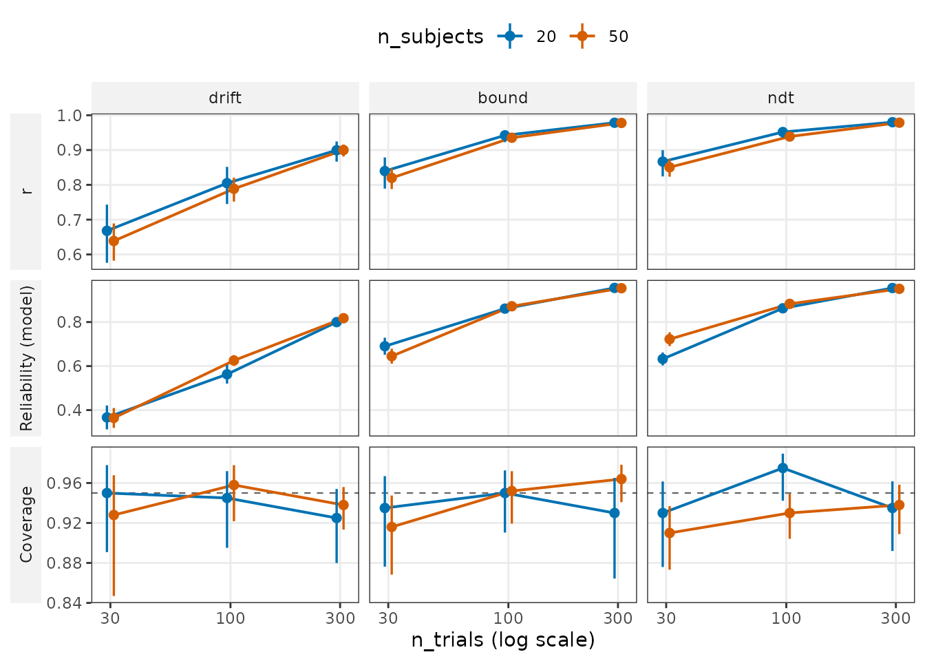

Here each person’s estimate is compared with that person’s generating value. The question is how well a study of this size ranks people, which is what an analysis of individual differences needs.

• r is, within one replication, the correlation between estimated and generating values across the people. The ten values of r are averaged after Fisher’s z transformation. Its bar runs from r_low to r_high, the usual 95 % interval of that average, tanh(z ± 1.96 / sqrt(N)) with N the sum of (people − 3) over the replications. r_low is the value the section “How many trials?” uses, because it is r with the uncertainty of ten replications taken off.
• Reliability (model) answers the same question without the truth, so a study can compute it on its own data: var(m) / (var(m) + mean(v)), with m the posterior means of the people and v their posterior variances, per replication and then averaged.
• Coverage is the share of all people’s 95 % CrIs that contain their generating value. It stays within 0.040 of 0.95 at every design.

bound and ndt are recovered well from 30 trials on (r ≥ 0.81). drift is the hard parameter: with 50 subjects its r is 0.64 at 30 trials, 0.79 at 100 and 0.90 at 300. More people do not make each person’s estimate detectably better: r is higher with 20 subjects than with 50 in 8 of the 9 comparisons at equal trials, the largest difference included, and at no design does r differ by more than 0.030 between 20 and 50 subjects, or by more than 1.5 standard errors of the difference. Ten replications would miss a true gain of less than 1.96 such standard errors more often than they would detect it, and that standard error is up to 0.051, for drift at 30 trials. From 100 trials on, with 20 subjects, the reliability from the model is nowhere above the squared correlation with the truth (in the table below) by more than 0.001, and below it by at most 0.074; with 50 it differs from it by at most 0.012. At 30 trials the gap reaches 0.090. So on data of that size from this model, it says how well the people are ranked, a little pessimistically with 20 subjects.

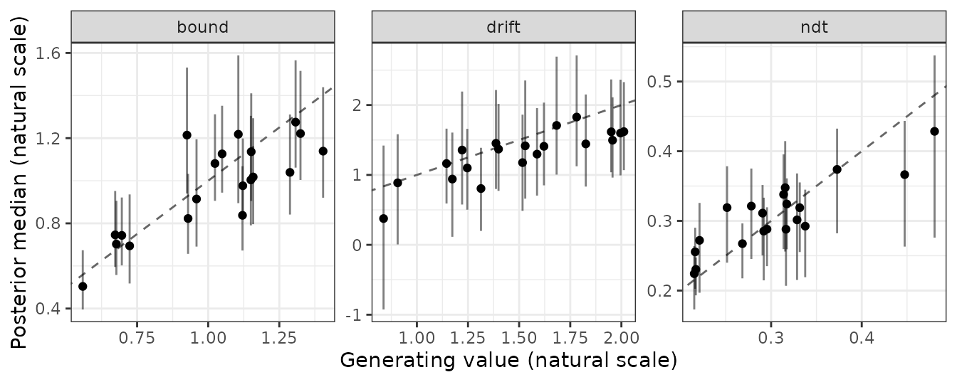
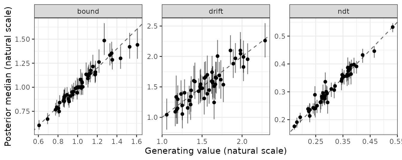
The two figures below show the first replication of the smallest and of the largest design: each person’s estimate against their generating value, on the natural scale (seconds for ndt), with the 95 % CrI. The dashed line is where estimate and truth are equal. These panels are in alphabetical order.

The subject numbers per design

Reliability from the truth is the squared correlation of m with the generating values; gap is the model’s reliability minus it, per replication, then averaged. Each is given with its MCSE, the SD over replications divided by √10.

subjects	trials	parameter	r	r_low	reliability from the truth	reliability from the model	gap
20	30	drift	0.67	0.58	0.44 ± 0.048	0.37 ± 0.054	-0.07 ± 0.047
20	30	bound	0.84	0.79	0.71 ± 0.026	0.69 ± 0.039	-0.02 ± 0.032
20	30	ndt	0.87	0.82	0.72 ± 0.028	0.63 ± 0.029	-0.09 ± 0.032
20	100	drift	0.80	0.75	0.64 ± 0.035	0.56 ± 0.042	-0.07 ± 0.053
20	100	bound	0.94	0.92	0.88 ± 0.020	0.86 ± 0.017	-0.02 ± 0.015
20	100	ndt	0.95	0.94	0.90 ± 0.010	0.86 ± 0.011	-0.04 ± 0.011
20	300	drift	0.90	0.87	0.80 ± 0.024	0.80 ± 0.017	-0.00 ± 0.013
20	300	bound	0.98	0.97	0.96 ± 0.007	0.96 ± 0.003	-0.00 ± 0.005
20	300	ndt	0.98	0.97	0.96 ± 0.008	0.95 ± 0.005	-0.00 ± 0.005
50	30	drift	0.64	0.58	0.41 ± 0.030	0.36 ± 0.045	-0.05 ± 0.036
50	30	bound	0.82	0.79	0.67 ± 0.021	0.64 ± 0.034	-0.03 ± 0.045
50	30	ndt	0.85	0.82	0.71 ± 0.029	0.72 ± 0.032	0.01 ± 0.033
50	100	drift	0.79	0.75	0.61 ± 0.028	0.63 ± 0.024	0.01 ± 0.016
50	100	bound	0.94	0.92	0.87 ± 0.011	0.87 ± 0.010	-0.00 ± 0.007
50	100	ndt	0.94	0.93	0.87 ± 0.005	0.88 ± 0.008	0.01 ± 0.008
50	300	drift	0.90	0.88	0.81 ± 0.013	0.82 ± 0.009	0.01 ± 0.013
50	300	bound	0.98	0.97	0.96 ± 0.004	0.95 ± 0.003	-0.00 ± 0.003
50	300	ndt	0.98	0.97	0.95 ± 0.004	0.95 ± 0.003	0.00 ± 0.003

The correlation between drift and boundary

plot_design(out, level = "correlation")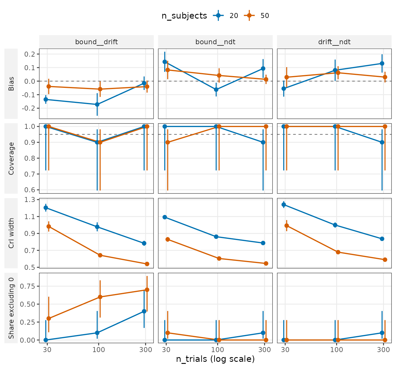

The simulation drew each person’s drift rate and boundary separation from a population in which they correlate 0.4 and left the other two pairs uncorrelated. A panel is named by the pair’s two parameters: bound__drift is the correlation between drift and boundary. Bias is the mean estimate minus the generating value, 0.4 or 0. Share excluding 0 is the share of replications whose 95 % CrI does not contain zero: for the 0.4 pair, the chance that a study of this size shows the correlation to differ from zero (its power).

The CrIs of the 0.4 correlation contain it in nine or ten of the ten replications at every design, but they are 0.54 to 1.20 wide, so they say little about its size. They exclude zero in at most 0.7 of the replications with 50 subjects and 0.4 with 20, both at 300 trials: even then, a study with 50 people missed a correlation of 0.4 between drift and boundary in 3 of 10 replications (Wilson interval of the miss rate 0.11 to 0.60). With 20 subjects and 30 trials the estimate is pulled towards zero (0.26 against an in-sample 0.51, the mean correlation of the values actually drawn; both are in the table below).

The correlation numbers per design

subjects	trials	pair	generating	in sample	mean estimate	covered	CrI width	CrI excludes 0
20	30	drift – bound	0.4	0.51	0.26	10/10	1.20	0.0
20	30	bound – ndt	0.0	0.08	0.14	10/10	1.09	0.0
20	30	drift – ndt	0.0	-0.04	-0.06	10/10	1.24	0.0
20	100	drift – bound	0.4	0.23	0.23	9/10	0.98	0.1
20	100	bound – ndt	0.0	-0.10	-0.06	10/10	0.86	0.0
20	100	drift – ndt	0.0	0.05	0.08	10/10	1.00	0.0
20	300	drift – bound	0.4	0.42	0.38	10/10	0.78	0.4
20	300	bound – ndt	0.0	0.14	0.09	9/10	0.79	0.1
20	300	drift – ndt	0.0	0.13	0.13	9/10	0.84	0.1
50	30	drift – bound	0.4	0.41	0.36	10/10	0.98	0.3
50	30	bound – ndt	0.0	-0.00	0.08	9/10	0.83	0.1
50	30	drift – ndt	0.0	0.04	0.03	10/10	0.99	0.0
50	100	drift – bound	0.4	0.43	0.34	9/10	0.64	0.6
50	100	bound – ndt	0.0	0.06	0.04	10/10	0.60	0.0
50	100	drift – ndt	0.0	0.12	0.06	10/10	0.68	0.0
50	300	drift – bound	0.4	0.38	0.36	10/10	0.54	0.7
50	300	bound – ndt	0.0	0.03	0.01	10/10	0.55	0.0
50	300	drift – ndt	0.0	0.04	0.03	10/10	0.59	0.0

How many trials?

Take a threshold for r_low, 0.80 by default, a common convention for measures used to rank individuals; 0.70 and 0.90 are given for readers with another threshold. The answer is the smallest number of trials at which r_low reaches the threshold for every parameter, and stays there at every larger number of trials in the grid.

One more condition: at that design, the coverage of every population mean must lie within one MCSE of 0.95, with the MCSE taken at 0.95, sqrt(0.95 × 0.05 / 10) = 0.069. With ten replications, 9 or 10 covered intervals out of 10 pass (0.90 is 0.05 from 0.95), and 8 or fewer fail (0.80 is 0.15 from it). Intervals of exactly the right width pass with probability 0.914, so a design whose 3 population means all have such intervals fails the condition with probability 0.24, if the 3 pass independently. A failure is weak evidence that the intervals are too narrow, but a design at which they are would be a poor recommendation, however well it ranks people. smallest_design() applies this rule to a grid summary:

s <- summary(out)
smallest_design(
  s[s$level %in% c("subject", "population"), ],
  c(r_low = 0.8),
  coverage_check = TRUE
)

It answers per parameter. The table below gives, for each number of subjects and threshold, the largest answer over the three parameters, the one that holds for every parameter. The column using r applies the threshold to r instead of r_low, without the coverage condition; the script computes it itself, because smallest_design() does not take r as a target. Where it is smaller, either r meets the threshold but ten replications are too few to be sure that it does, or the coverage condition moved the answer up.

subjects	bar	smallest number of trials	using r
20	0.70	100	100
20	0.80	300	100
20	0.90	not reached in this grid	not reached in this grid
50	0.70	300	100
50	0.80	300	300
50	0.90	not reached in this grid	300

With 50 subjects and bmm 1.4.1, a study needs 300 trials per person for an r_low of at least 0.80 on every parameter. The grid has nothing between its trial counts, so “300” means more than 100 and at most 300. The answers in this section hold at the generating values of this study, chiefly drift’s between-subject SD of 0.3 on the link scale: r and the reliability compare how much people differ with how precisely each is estimated, so where people differ more or less, the answer can change. drift decides the r_low part of each answer: at 100 trials its r_low is 0.75, at 300 0.88. That is also why 0.90 is not reached: drift’s r at 300 trials, 0.900005, meets it only in the sixth decimal (the 300 under using r), and its r_low does not. The 0.80 answer is safe on r_low but not on coverage: bound covered in 9/10 replications at that design, and one more miss would turn the answer into “not reached in this grid”.

The answer at 0.70 shows how much ten replications can decide. By r_low alone it is 100 trials. But at that design bound covered in 8/10, so the rule moves on to 300 trials. With one more covered interval the answer would have been 100, and the second run of this script (see “The run”), with different starting values, gave exactly that. Read it as “100 or 300”.

The number of subjects does not change the r_low part of these answers: by r_low alone, 20 subjects need 100 trials at 0.70 and 300 at 0.80, as 50 do. More people narrow the interval of r and of the population estimates; they do not measure each person detectably better. At the 0.80 threshold, r alone would say 100 trials with 20 subjects: drift’s r there is 0.80, but its r_low is 0.75.

Reproducing the study

vignettes/articles/precompute/recovery-ezdm.R runs the grid and writes the results this page reads, to vignettes/articles/assets/recovery-ezdm.rds. It needs bmm 1.4.1 or later, brms, cmdstanr and CmdStan, and a copy of the bmmtools source. Run it from the package’s root folder with Rscript vignettes/articles/precompute/recovery-ezdm.R; it took 9 minutes for the run shown here, four chains in parallel. The fitted models go to vignettes/articles/precompute/fits/.