Plot recovery across the designs of a grid

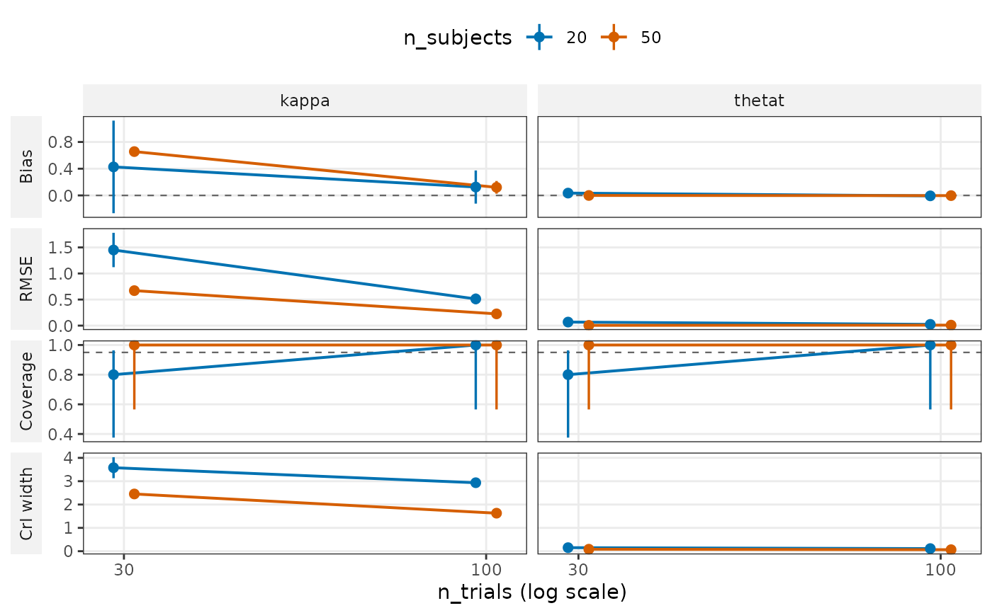
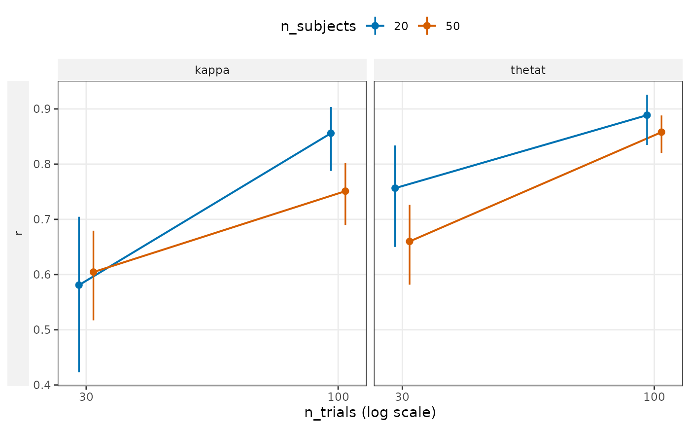
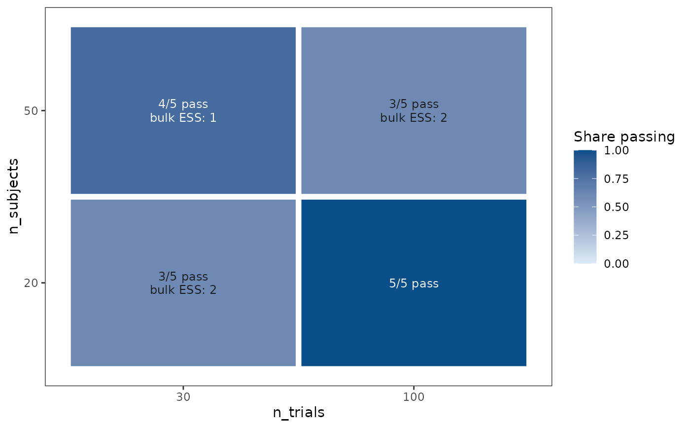
The picture a grid summary is read through: how a metric changes with the design. type = "profile" puts a metric on the y axis against trials per subject (a log axis), one line per number of subjects and a panel per term and metric. type = "convergence" draws one tile per design with the share of fits that passed the convergence gate and the checks the others failed. type = "coverage" pools the intervals of every design per term and level, the coverage check that does not depend on ten replications per design. plot_recovery() shows the estimates of one design against their truth.

Usage

plot_design(x, ...)

# Default S3 method
plot_design(x, ...)

# S3 method for class 'bmmtools_recovery'
plot_design(
  x,
  type = c("profile", "convergence", "coverage"),
  level = "population",
  metric = NULL,
  x_axis = "n_trials",
  color_by = "n_subjects",
  ...
)

# S3 method for class 'bmmtools_recovery_summary'
plot_design(
  x,
  type = "profile",
  level = "population",
  metric = NULL,
  x_axis = "n_trials",
  color_by = "n_subjects",
  ...
)

Arguments

x: A bmmtools_recovery object from recovery_grid(), or its summary(). A summary draws profiles only.
...: Not used.
type: "profile", "convergence" or "coverage".
level: For a profile, the level to draw: "population", "sd", "subject", or "correlation" for the model correlations a grid run with correlations carries.
metric: For a profile, the summary columns to draw, one panel row each, in this order. NULL draws bias, RMSE, coverage and CrI width for population means and SDs; r, the model-based reliability and coverage for subjects; bias, coverage, CrI width and the share of intervals excluding zero for correlations. "pass_rate" and "fit_seconds" come from the grid's cells and are drawn without level and without the other metrics.
x_axis, color_by: Design columns of the grid: the one on the x axis and the one that makes the lines (the rows and columns of the convergence tiles).

Value

A ggplot object. Its data holds the numbers drawn, with the bars in lower and upper.

Details

A filter on x reaches the profiles of its rows and the model correlations. The convergence tiles and the cell metrics draw the designs x holds and count every replication of them: an errored fit has no rows, so a filter on replications or on converged cannot be read back from x, and a message says so. A design without rows (every fit errored, or every fit in the replications x holds) is still drawn, unless x was filtered by condition to designs whose values it does not share; a message names it then. A filter that removes every row of a design that ran in those replications removes its tile.

A figure refuses a design column named like a column it is drawn from: value, lower, upper, metric or colour_group in a profile, pass, label or dark in the tiles, status, converged, failed or fit_seconds in the tiles and the cell metrics, and a column of the correlation summary at the correlation level. Rename it in the grid.

Error bars

Each metric's bar has one source, stated here so that a figure can be read without the code:

bias: ±1 Monte Carlo standard error (MCSE), the SD of the errors over the replications / sqrt(R) (Morris et al., 2019, Table 6). None at the subject level, where the errors of one replication are not independent.
rmse: ±1 MCSE of the MSE (Morris et al., 2019, Table 6) carried to the RMSE by the delta method, MCSE(MSE) / (2 RMSE). Not at the subject level.
ci_width, ci_width_50, contraction: ±1 MCSE, the SD of the replications' means / sqrt(R).
Rates (coverage, coverage_50, detected, sign_recovery, rejection_rate, pass_rate, ...): a 95 % Wilson score interval, which stays inside 0 to 1 and is not empty at a rate of 1. The count is the number of replications that entered the rate (for sign recovery, those whose truth is not zero); from a summary, which has dropped them, its complete pairs. At the subject level it is the count behind the between-replication MCSE that summary() reports (the effective n of smallest_design()), or the replications at a rate of 0 or 1. A subject rate of exactly 0 or 1 has a between-replication MCSE of 0, which carries no count, so the interval at the replications is conservative: it can be much wider than at a rate just below 1.
r: the pooled interval r_low to r_high of summary().
reliability_model, reliability_true, reliability_gap, z_mean, z_sd: ±1 of the MCSE column summary() reports. At the subject level that MCSE counts every subject as independent and understates, so z_mean takes ±1 MCSE, the SD of the replications' mean z / sqrt(R), and z_sd has no bar: it pools the subjects of every replication, so it also holds the spread between their mean z, which a bar from the replications' own SDs would leave out.
fit_seconds: ±1 MCSE, the SD over fits / sqrt(fits).

Any other metric is drawn without a bar. From a summary, which has dropped the replications, rmse, the widths, contraction and the subject-level z_mean have no bar.

References

Morris, T. P., White, I. R., & Crowther, M. J. (2019). Using simulation studies to evaluate statistical methods. Statistics in Medicine, 38(11), 2074–2102. doi:10.1002/sim.8086

Examples

# population means across the four designs of the example grid
plot_design(recovery_mixture2p)


# subject parameters, and r alone
plot_design(recovery_mixture2p, level = "subject", metric = "r")


# how many fits passed the convergence gate, per design
plot_design(recovery_mixture2p, type = "convergence")